Automation in process control 2nd Module

Controller Principles

Process characteristics

The selection of what controller modes to use in a process is a function of the characteristics of the process. It is not our intention to discuss how the modes are selected but to define the meaning of each mode. At the same time, it is helpful in understanding the modes if certain pertinent characteristics of the process are considered. In this section, we will define a few properties of processes that are important for selecting the proper mode

Process Equation

A process-control loop regulates some dynamic variable in a process. This controlled variable, a process parameter, may depend on many other parameters (in the process) and thus suffer changes from many different sources. We have selected one of these other parameters to be our controlling parameter.

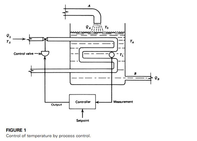
If a measurement of the controlled variable shows a deviation from the setpoint, then the controlling parameter is changed, which in turn changes the controlled variable. As an example, consider the control of liquid temperature in a tank, as shown in Figure 1.

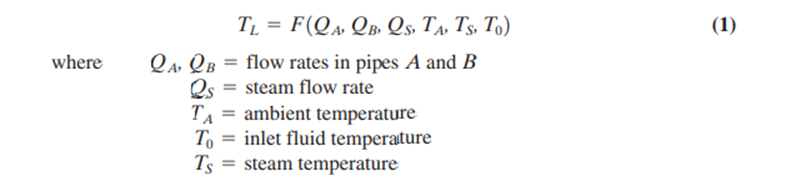
The controlled variable is the liquid temperature, This temperature depends on many parameters in the process—for example, the input flow rate via pipe A, the output flow rate via pipe B, the ambient temperature, , the steam temperature, , inlet temperature, , and the steam flow rate, .

In this case, the steam flow rate is the controlling parameter chosen to provide control over the variable (liquid temperature). If one of the other parameters changes, a change in temperature results. To bring the temperature back to the setpoint value, we change only the steam flow rate—that is, heat input to the process. This process could be described by a process equation where liquid temperature is a function as

Process Load

From the process equation, or knowledge of and experience with the process, it is possible to identify a set of values for the process parameters that results in the controlled variable having the setpoint value. This set of parameters is called the nominal set. The term process load refers to this set of all parameters, excluding the controlled variable

When all parameters have their nominal values, we speak of the nominal load on the system. The required controlling variable value under these conditions is the nominal value of that parameter. If the setpoint is changed, the control parameter is altered to cause the variable to adopt this new operating point. The load is still nominal, however, because the other parameters are assumed to be unchanged. Suppose one of the parameters changes from nominal, causing a corresponding shift in the controlled variable. We then say that a process load change has occurred.

In the example of Figure 1, a process load change is caused by a change in any of the five parameters affecting liquid temperature. The extent of the load change on the controlled variable is formally determined by process equations such as Equation (1).

Transient Another type of change involves a temporary variation of one of the load parameters. After the excursion, the parameter returns to its nominal value. This variation is called a transient. A transient causes variations of the controlled variable, and the control system must make equally transient changes of the controlling variable to keep error to a minimum. A transient is not a load change because it is not permanent.

Process Lag

As previously noted, process-control operations are essentially a time-variation problem. At some point in time, a process-load change or transient causes a change in the controlled variable. The process-control loop responds to ensure that, some finite time later, the variable returns to the setpoint value. Part of this time is consumed by the process itself and is called the process lag.

Thus, referring to Figure 1, assume the inlet flow is suddenly doubled. Such a large process-load change radically changes (reduces) the liquid temperature. The control loop responds by opening the steam inlet valve to allow more steam and heat input to bring the liquid temperature back to the setpoint. The loop itself reacts faster than the process.

In fact, the physical opening of the control valve is the slowest part of the loop. Once steam is flowing at the new rate, however, the body of liquid must be heated by the steam before the setpoint value is reached again. This time delay or process lag in heating is a function of the process, not the control system. Clearly, there is no advantage in designing control systems many times faster than the process lag

Self-Regulation

A significant characteristic of some processes is the tendency to adopt a specific value of the controlled variable for nominal load with no control operations. The control operations may be significantly affected by such self-regulation.

The process of Figure 1 has self regulation, as shown by the following argument. (1) Suppose we fix the steam valve at 50% and open the control loop so that no changes in valve position are possible. (2) The liquid heats up until the energy carried away by the liquid equals that input energy from the steam flow. (3) If the load changes, a new temperature is adopted (because the system temperature is not controlled). (4) The process is self-regulating, however, because the temperature will not “run away,” but stabilizes at some value under given conditions

Control system parameters

Error

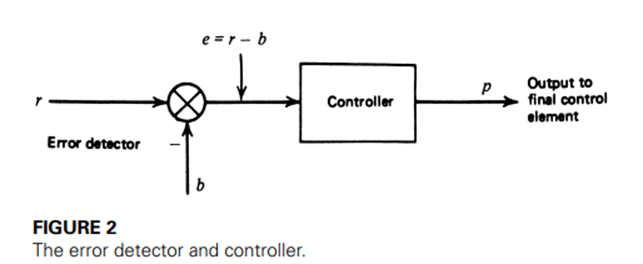
Error is the difference between the measured variable and the setpoint. Error can be either positive or negative. The objective of any control scheme is to minimize or eliminate error. The deviation or error of dynamic variable from set point is given by:

E = r-b (2)

Where E = error

b = measured value of variable

r = set point of variable

The above equation expresses error in an absolute sense, usually in units of measured analog of control signal. Note that a positive error indicates a measurement above the set points whereas a negative error indicates a measurement below the set point.

Variable range

The dynamic variable under control or controlled variable has a range of values within which control is required to be maintained at set point. This range can be expressed as the minimum and maximum values of the dynamic variable or the nominal value plus and minus the spread about this nominal value e.g. if a standard signal 4-20 mA transmission is employed, then 4 mA represents the minimum value of the variable and 20 mA the maximum value.

Control parameter (output) range

It is the possible range of values of final control element. The controller output is expressed as a percentage where minimum controller output is 0% and maximum controller is 100%. But 0% controller output does not mean zero output. For example, it is necessary requirement of the system that a steam flow corresponds to 1/4^th opening of valve. The controller parameter output has a percentage of full scale when the output changes within the specified limits in expressed as:

Where:

P = Controller output as percentage of full scale

u = Value of the output

u_max = Maximum value of the controlling parameter

u_min = Minimum value of the controlling parameter

Control lag

Processes have the characteristic of delaying and retarding changes in the values of the process variables.  This characteristic greatly increases the difficulty of control. The control system can have a lag associated with it. The control lag is the time required by the process and controller loop to make the necessary changes to obtain the output at its set point.

The control lag must be compared with process lag while designing the controllers. A process time lag is the general term that describes the process delays and retardations. It refers to the time for the process control loop to make necessary adjustments to the final control element e.g. if a sudden change in liquid temperature occurs, it requires some finite time for the control system to physically actuate the steam control valve.

Dead time

Sometimes a dead zone is associated with the process control loop. The time corresponding to dead zone is called dead time. This is the elapsed time between the instant a deviation (error) occurs and when the corrective action first occurs.

Cycling

We frequently refer to the behavior of the dynamic variable error under various modes of control. One of the most important modes is an oscillation of the error about zero. This means the variable is cycling above and below the setpoint value. Such cycling may continue indefinitely, in which case we have steady-state cycling.

Controller Modes

The method used by the controller to correct the error is the control mode. Controller modes are an expression of relation between controller output and dynamic variable deviation from the set point. The actions of controllers can be divided into groups based upon the functions of their control mechanism. Each type of controller has advantages and disadvantages and meets the needs of different applications. Grouped by control mechanism function, the two types of controllers are:

1.      Discontinuous controllers

2.      Continuous controllers

Discontinuous control mode

In this mode controller command initiates a discontinuous change in control parameter. The manipulated variable of a discontinuous controller mode can only be changed in set steps. The best-known discontinuous-action controller is the two-step control that can only assume the conditions on or off. An example is the thermostat of a hot air oven. It switches the electric current for the heating element on or off depending on the set temperature.

Types of discontinuous controller modes

The choice of operating modes for any given process control system is a complicated decision. It involves not only process characteristics but cost analysis, product rate, and other industrial factors. The different types of discontinuous controller operating modes are defined as follows:

(A) Two Position Controller Mode:  A  two  position controller mode uses a  device  that  has  two operating  conditions: completely  on  or completely off. These also called ON-OFF control or Discrete controllers. On /off control activates an output until the measured value reaches the reference value. Fig. 28.1 shows the input to output characteristic for a two position controller for a refrigerator that switches from its OFF to its ON state when the measured variable increases above the set point.

Conversely,  it  switches from  its  ON  state  to  its OFF  state  when  the  measured variable decreases below the set point.  This device provides an output determined by whether the error signal is above or below the set point. The magnitude of the error signal is above or below the set point. The magnitude of the error signal past that point is of no concern to the controller.

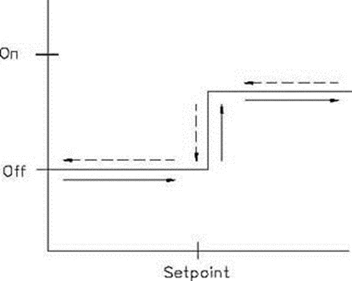
Fig. 28.1  Two position controller input/output relationship

While simple and low cost, this mode of control has a tendency to overshoot the desired value. Flow Diversion Valve (FDV) used in HTST plant and solenoid valves are two position ON-OFF controller.

(B) Multi-position Mode or Multistep Mode Controllers

Multistep controllers are controllers that have at least one other possible position in addition to on and off. Multistep controllers operate similarly to discrete controllers, but as set-point is approached, the multistep controller takes intermediate steps.

Therefore, the oscillation around set-point can be less dramatic when multistep controllers are employed than when discrete controllers are used. This mode is used to provide several intermediate values rather than only two settings of controller output.

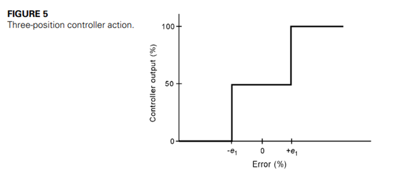
This discontinuous control mode is used to reduce the cycling behaviour and also overshoot and undershoot inherent in two position control. This mode is represented by:

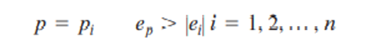
The meaning here is that as error exceeds certain set limits + Ei, the controller output is adjusted to preset values Pi. The most common example is the three-position controller where

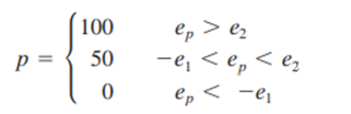
Figure 5 illustrates this mode graphically. Some small neutral zone usually exists about the change points, but not by design; thus, it is not shown.

(C) Floating Control Modes

In this control mode, specific output of the controller is not uniquely determined by error. If error is zero, the output will not change but remains (floats) at whatever settings it was when the error went to zero. When the error moves off zero, the controller output begins to change e.g. a floating control will operate a control valve which, as level rises and falls will throttle down or gradually open a level control valve in the inlet (or outlet) line, thereby controlling the level at a pre-set height in the tank.

Single Speed In the single-speed floating-control mode, the output of the control element changes at a fixed rate when the error exceeds the neutral zone. An equation for this action is

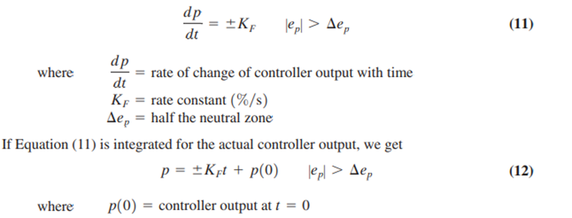
A graph of single-speed floating control is shown in Figure 7a.

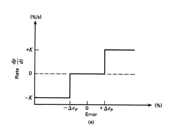
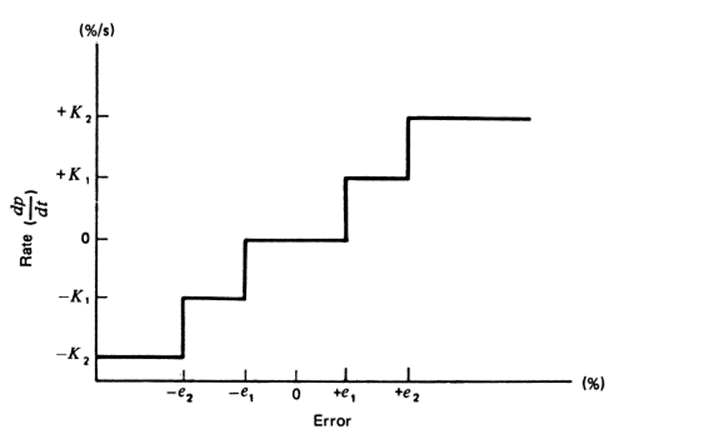
Multiple Speed In the floating multiple-speed control mode, not one but several possible speeds (rates) are changed by controller output. Usually, the rate increases as the deviation exceeds certain limits. Thus, if we have certain speed change points, e_pi depending on the error, then each has its corresponding output rate change,K_i We can then say

If the error exceeds e_pip, then the speed is K_Fi. If the error rises to exceed e_p2, the speed is increased to K_F2, and so on. Actually, this mode is a discontinuous attempt to realize an integral mode.

A graph of this mode is shown in Figure 8. Applications Primary applications of the floating-control mode are for the single-speed controllers with a neutral zone.

Continuous control modes

Proportional Control Mode

In the proportional (throttling) mode, there is a continuous linear relation between value of the controlled variable and position of the final control element. In this control mode, the output of the controller is proportional to error e(t). The relation between the error e(t) and the controller output p is determined by a constant called proportional gain constant denoted as K_p. The output of the controller is a linear function of e(t).

p(t) = K_pe(t) + p(0)                                     (1)

Where:

K_p = Proportional gain constant

P(0) = Controller output with zero error or bias

The direct and reverse action is possible in the proportional controller mode. The error may be positive or negative because error (r-b) depending upon whether b is less or greater than the reference setpoint r(t).

If the controlled variable i.e. input to the controller increases, causing increase in the controller output, the action is called direct action. For example the output valve is to be controlled to maintain the liquid level in a tank. If the level increases, the valve should be opened more to maintain the level. On the other hand if the variable decreases, causing increase in the controller output, the action is called reverse action. Conversely, increase in the controlled variable, causing decrease in controller output is also a reverse action.

29.1.1 Characteristics of proportional mode

The various characteristics of the proportional mode are:

1.      When the error is zero, the controller output is constant equal to p_0.

2.      If the error occurs, then for every 1 % of error the correction of K_p % is achieved. If error is positive, K_p % correction gets added to p₀ and if error is negative, K_p % correction gets subtracted from p₀.

3.      The band of error exists for which the output of the controller is between 0 to 100%.

4.      The gain K_p and error band PB are inversely proportional to each other.

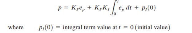
Integral Control Mode

With integral action, the controller output is proportional to the amount of time the error is present. Integral action eliminates offset that remains when proportional control is used. In such a controller, the value of the controller output p(t) is changed at a rate which is proportional to the actuating error signal e(t). Mathematically it is expressed as:

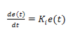
Where K_i = constant relating error and rate

The constant K_i is also called integral constant. Integrating the above equation, the actual output at any time t can be obtained as

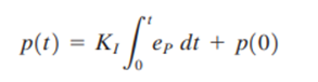
Where p(0) = controller output when integral action starts i.e. at t = 0.

Advantages

1.      Integral controllers tend to respond slowly at first, but over a period of time they tend to eliminate errors.

2.      The integral controller eliminates the steady-state error, but has the poor transient response and leads to instability.

Characteristics of integral mode

1.      If error is zero, the output remains at a fixed value equal to what it was, when the error become zero.

2.      If the error is not zero, then the output begins to increase or decrease, at a rate Ki % per second for every 1 % of error.

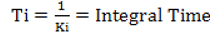
3.      The inverse of Ki is called integral time and denoted as Ti.

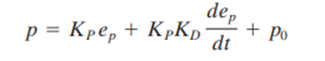
Derivative Control Mode

In this mode, the output of the controller depends on the rate of change of error. Hence, it is also called rate action mode or anticipatory action mode. The mathematical equation for the mode is:

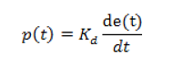
Where Kd = Derivative gain constant

The derivative gain constant indicates by how much % the controller output must change for every % per second rate of change of the error. Generally Kd is expressed in minutes. The important feature of this type of control mode is that for a given rate of change or error signal, there is a unique value of the controller output.

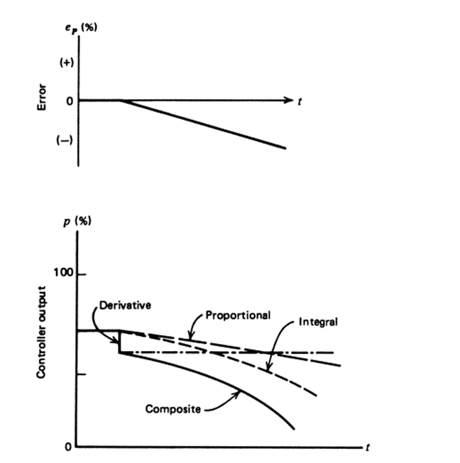
The advantage of the derivative control action is that it responds to the rate of change of error and can produce the significant correction before the magnitude of the actuating error becomes too large. Derivative control thus anticipates the actuating error, initiates an early corrective action and tends to increase stability of the system, improving the transient response. The derivative or differential controller is never used alone because when error is zero or constant, the controller has either no output or the nominal output for zero error.

Characteristics of derivative control mode

For a given rate of change of error signal, there is a unique value of the controller output. When the error is zero, the controller output is zero. When the error is constant i.e. rate of change of error is zero, the controller output is zero. When the error is changing, the controller output changes by K_d % for even 1 % per second rate of change of error.

When the error is zero or a constant, the derivative controller output is zero. Hence, it is never used alone. Its gain should be small because faster rate of change of error can cause very large sudden change of controller output. This may lead to instability of the system.

Composite control mode

P-I (proportional and integrative) control mode:

A P-I controller accumulates the error as time passes and is multiplied by the constant Ki. That is your term. It outputs the sum of your P and I terms. PI controllers have two adjustment parameters to adjust. The integral action allows the PI controllers to eliminate the offset, a major weakness of a P-only controller. Therefore, PI controllers provide a balance of complexity and capacity that makes them the most used algorithm in process control applications. This driver is used mainly in areas where system speed is not a problem. Since the P-I controller does not have the ability to predict future system errors, it can not decrease the rise time and eliminate oscillations.

The analytic expression for this control process is

P-D (proportional-derivative) controller mode:

The objective of using the P-D controller is to increase the stability of the system by improving the control since it has the ability to predict the future error of the system response. This system can not eliminate the displacement of the proportional controllers, however, it can handle rapid process load changes as long as the load change compensation error is acceptable.

The D mode is designed to be proportional to the change of the output variable to avoid the sudden changes that occur in the control output as a result of sudden changes in the error signal. In addition, D directly amplifies the process noise, so the D-only control is not used.

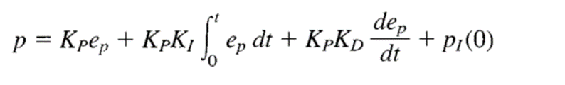
P-I-D Controller (Three-Mode Controller):

The P-I-D controller has the optimal control dynamics that include zero steady-state error, fast response (short rise time), no oscillations and greater stability. With the addition of a third parameter adjustable adjustment derivative, the number of algorithm permutations increases markedly. And there are even different forms of the PID equation itself. This creates additional challenges for the design and adjustment of the driver. One of the main advantages of the P-I-D controller is that it can be used with higher order processes that include more than individual energy storage.

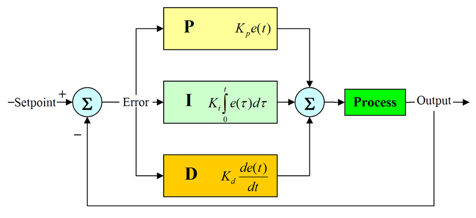
The time response of the controlled variable can be modified by adjusting the proportional gain K, and the integrating and derivative time constants Ti and Td, respectively; the objective is to achieve a zero steady state control error e (t) regardless of whether it is caused by changes in the reference  or the perturbation d(t).

The analytic expression includes the expression of the three parameters: