Automation in process control 3rd Module

DISCRETE-STATE PROCESS CONTROL:

Definition and characteristics of discrete state process control

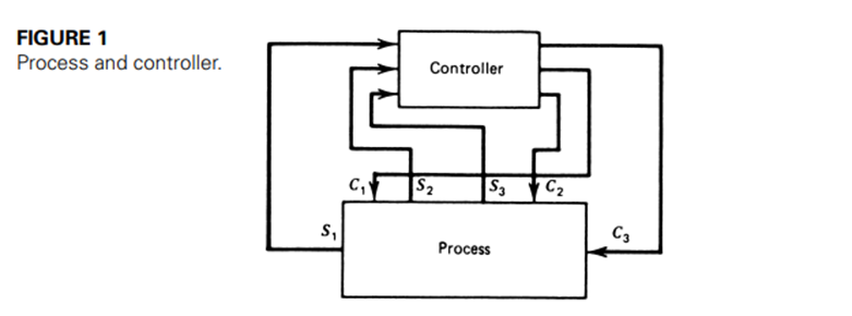
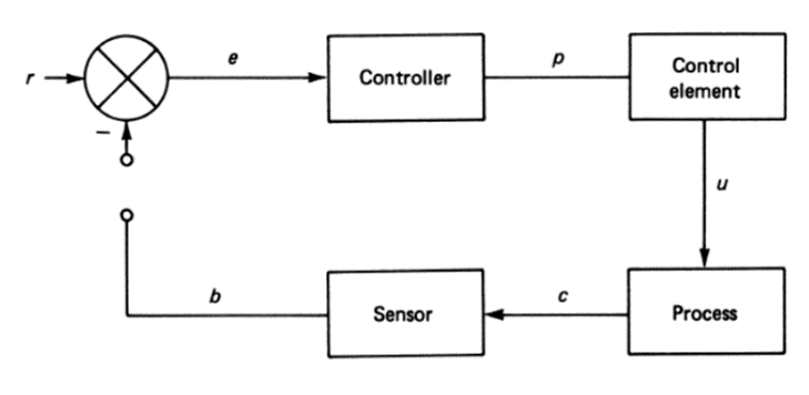
Figure 1 is a symbolic representation of a manufacturing process and the controller for the process. Let us suppose that all measurement input variables (S₁,S₂,S₃) and all control output variables (C₁,C₂,C₃)  of the process can take on or be assigned only two values.

For example, valves are open/closed, motors are on/off, temperature is high/low, limit switches are closed/open, and so on. Now we define a discrete state of the process at any moment to be the set of all input and output values. Each state is discrete in the sense that there is only a discrete number of possible states. If there are three input variables and three output variables, then a state consists of specification of all six values.

Because each variable can take on two values, there is a total of 64 possible states. An event in the system is defined by a particular state of the system—that is, particular assignment of all output values and a particular set of the input variables. The event lasts for as long as the input variables remain in the same state and the output variables are left in the assigned state.

For a simple oven, we can have the temperature low and the heater on. This state is an event that will last until the temperature rises. With these definitions in mind, discrete-state process control is a particular sequence of events through which the process accomplishes some objective. For a simple heater, such a sequence might be

1. Temperature low, heater off

2. Temperature low, heater on

3. Temperature high, heater on

4. Temperature high, heater off

The objective of the controller of Figure 1 is to direct the discrete-state system through a specified event sequence. In the following sections, we will consider how the event sequence is specified, how it is described, and how a controller can be developed to direct the sequence of events.

Characteristics of system

The objective of an industrial process-control system is to manufacture some product from the input raw materials. Such a process will typically involve many operations or steps. Some of these steps must occur in series and some can occur in parallel.

Some of the events may involve the discrete setting of states in the plant—that is, valves open or closed, motors on or off, and so on. Other events may involve regulation of some continuous variable over time or the duration of an event.

For example, it may be necessary to maintain the temperature in some vat at a setpoint for a given length of time. In the sense of the previous statements, the discrete state process-control system is the master control system for the entire plant operation

The characteristics are described by “Discrete State Variables”, “Process Specifications” & “Event Sequence Descriptions”

Discrete-State Variables

It is important to be able to distinguish between the nature of variables in a discrete-state system and those in continuous control systems.

• To define the difference carefully, we will consider an example contrasting a continuous variable situation with a discrete-state variable situation for the same application.

• It can be shown that continuous variable regulation can be itself a part of a discrete-state system. It can be viewed from the point of view of continuous control, discrete-state control and composite control.

i) Continuous Control

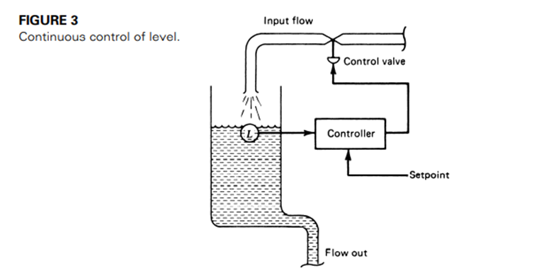
• Consider for a moment the problem of liquid level in a tank. Figure shows a tank with a valve that controls flow of liquid into the tank and some unspecified flow out of the tank.

• A transducer is available to measure the level of liquid in the tank. Also shown is the block diagram of a control system whose objective is to maintain the level of liquid in the tank at some preset or setpoint value.

• The controller will operate according to some mode of control to maintain the level against variations induced from external influences.

• Thus, if the outflow increases, the control system will increase the opening of the input valve to compensate by increasing the input flow rate.

• The level is thus regulated. This is a continuous variable control system because both the level and the valve setting can vary over a range.

• Even if the controller is operating in an ON/OFF mode, there is still variable regulation, although the level will now oscillate as the input valve is opened and closed to compensate for output flow variation.

iii) Composite Discrete/Continuous Control

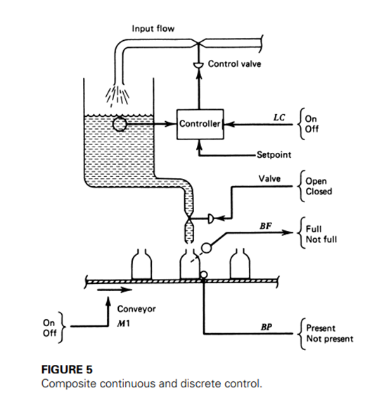
• It is possible for a continuous control system to be part of a discrete-state process-control system. As an example, consider

• the problem of the tank system described in Continuous Control. In this case, we specify that the outlet valve is to be closed and the tank filled to the required level as in Discrete State Control.

• We now specify, however, that periodically a bottle comes into position under the outlet valve, as shown in Figure shown.

• The level must be maintained at the setpoint while the outlet valve is opened, and the bottle filled. This requirement may be necessary to ensure a constant pressure head during bottle filling.

• This process will require that a continuous-level control system be used to adjust the input flow rate during bottle-fill through the output valve.

• The continuous control system will be turned on or off just as would a valve or motor or other discrete device.

• You can see that the continuous control process is but a part of the overall discrete-state process.

Process Specifications

Specification of the sequence of events in some discrete-state process is directly tied to the process itself. The process is specified in two parts. The first part consists of the objectives of the process, and the second is the nature of the hardware assembled to achieve the objectives.

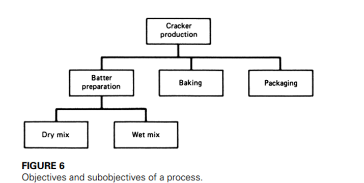
• Process Objectives The objectives of the process are simply statements of what the process is supposed to accomplish. Objectives are usually associated with knowledge of the industry. Often a global objective is defined as the end result of the plant. This is then broken down into individual, mostly independent secondary objectives to which the actual control is applied.

For example, in a food industry plant, a particular global objective might be to produce crackers. Clearly, this means that the plant takes in raw materials, processes them in specified ways, and outputs packaged and labeled crackers, ready for sale.

The overall objective can be broken down into many secondary objectives. Figure suggests some of the secondary objectives that might be involved.

Process Hardware

With determination of the objectives of the process comes the design of hardware to implement these objectives. This hardware is closely tied to the nature of the industry, and its design must come from the joint efforts of process, production, and control personnel. For the control system specialist, the essential thing is to develop a good understanding of the nature of the hardware and its characteristics.

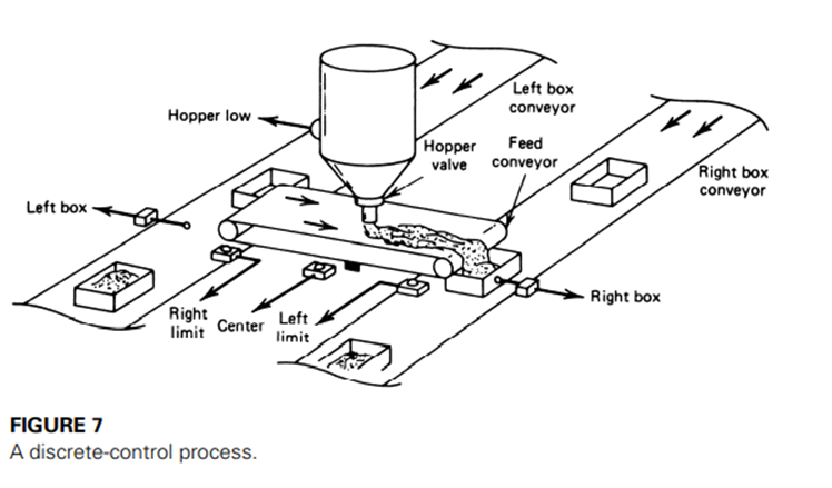
Figure 7 shows a pictorial representation of process hardware for a conveyor system. The objective is to fill boxes moving on two conveyors from a common feed hopper and material-conveyor system. A process-control system specialist may not have been involved in the development of this system.

To develop the control system, he or she must study the hardware carefully and understand the characteristics of each element. In general, the specialist analyzes the hardware by considering how each part is related to the control system. There are really only two basic categories

1.Input devices provide inputs to the control system. The operation of these devices is similar to the measurement function of continuous control systems. In the case of discrete-state process control, the inputs are two-state specifications, such as

Limit switches: open or closed

Comparators: high or low

Push buttons: depressed or not depressed

2. Output devices accept output commands from the control system. The final control element of continuous control systems does the same thing. In discretestate process control, these output devices accept only two-state commands, such as

Light: on or off

Motor: rotating or not rotating

Solenoid: engaged or not engaged

Event Sequence Description

Now that the subobjectives of a process and the necessary hardware have been defined, the job remains to describe how this hardware will be manipulated to accomplish the objective. A sequence of events must be described that will direct the system through the operations to provide the desired end result. Narrative Statements Specification of the sequence of events starts with narrative descriptions of what events must occur to achieve the objective. In many cases, this first attempt at specification reveals modifications that must be made in the hardware, such as extra limit switches. This specification describes in narrative form what must happen during the process operation. In systems that run continuously, there are typically a startup, or initialization, phase and a running phase.

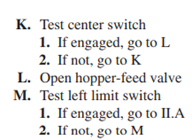
As an example, consider the system described by Figure 7. The start-up phase is used to place the feed conveyor in a known condition. This initialization might be accomplished by the following specification: I. Initialization Phase A. All motors off, feed valve solenoid off B. Test for right limit switch

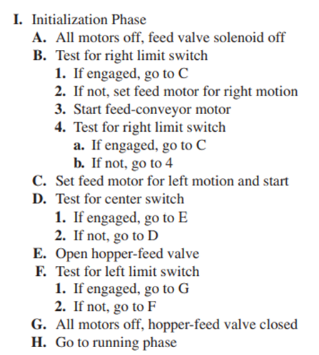
Completion of this phase means that the feed conveyor is positioned at the left limit position and the right half of the conveyor has been filled from the feed hopper.

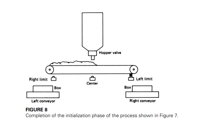
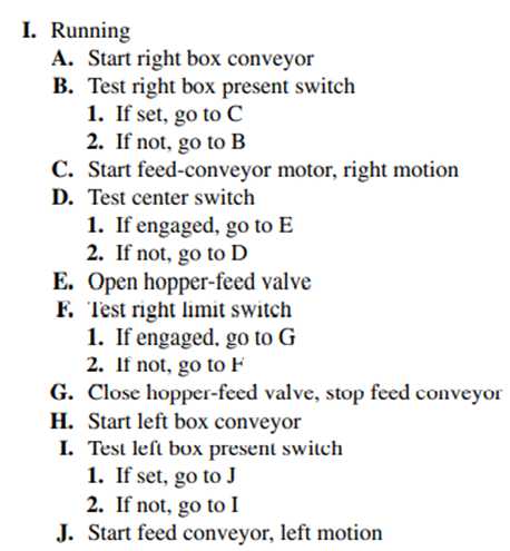
The system is in a known configuration, as shown in Figure 8. The running phase is described by a similar set of statements of the sequence of events. For the example of Figure 7, this phase might be described as follows:

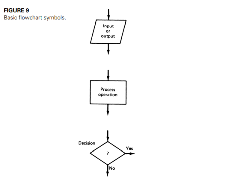
Flowcharts of the Event Sequence

It is often easier to visualize and construct the sequence of events if a flowchart is used to pictorially present the flow of events. Although there are many sophisticated types of flowcharts, the concept can be presented easily by using the three symbols shown in Figure 9

The narrative statements are then simply reformatted into flowchart symbols. Often it is easier to express the sequence of events directly in terms of the flowchart symbols.

Binary-State Variable Descriptions

Each event that makes up the sequence of events described by the narrative scheme corresponds to a discrete state of the system. Thus, it is also possible to describe the sequence of events in terms of the sequence of discrete states of the system. To do this simply requires that for each event the state, including both input and output variables, be specified.

The input variables cause the state of the system to change because operations within the system cause a change of one of the state variables; for example, a limit switch becomes engaged. The output variables, in contrast, are changes in the system state that are caused by the control system itself.

The control system works like a look-up table. The input state variables with the output become like a memory address, and the new output state variables are the contents of that memory

Boolean Equations

Because the discrete state of the system is described by variables that can take on only two values, it is natural to think of using binary numbers to represent these variables, as in the previous example. It is also natural to consider use of Boolean algebra techniques to deduce the output states from the input states. Although this technique is used, there are generally easier ways to view and solve the problems than with traditional Boolean techniques.

When this technique is used, it is necessary to write a Boolean equation for each output variable in the system. This equation will then determine when that variable is taken to its true state. The equation may depend not only on the set of input variables, but on some of the other output variables.

Control-loop characteristics:

Control system configuration

➢We consider first, the types of control-loop configurations that are encountered in typical industrial applications.

➢The control-loop concept is a correct one, but necessarily oversimplifies many of the actual configurations used in industry.

➢The decision of which arrangement to select is made by the process designers based on the goal of the process relative to production requirements, and the physical characteristics of operations under control.

Single Variable:

• The elementary process-control loop is a single-variable loop. The loop is designed to maintain control of a given process variable by manipulation of a controlling variable, regardless of the other process parameters.

Independent Single Variable: In many process-control applications, certain regulations are required regardless of other parameters in the process. In these cases, a set point is established, controller action is started, and the system is left alone.

Thus, in Figure, a flow-control system is used to regulate flow into a tank at a fixed rate determined by the set point. This system then makes adjustments in valve positions as necessary following a load change to maintain flow rate at the set point value.

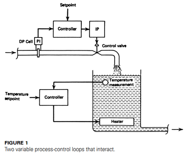
Interactive Single Variable A second single-variable control loop, shown in figure, regulates the temperature of liquid in the tank by adjustment of heat input. This also is a single-variable loop that maintains the liquid temperature at the setpoint value.

• Under nominal conditions, the flow into the tank is held constant and the temperature is also held constant, both at their respective setpoint values. Note, however, that a change in the setpoint of the flow-control system appears as a load change to the temperature-control system, because the fluid level in the tank or rate of passage through the tank must change.

• The temperature system now responds by resetting the heat flux to accommodate the new load and bring the temperature back to the setpoint. We say, then, that these two loops interact.

• Almost any process where several variables are under control shows such interactive behavior. Any cycling or other instability of the flow-control loop causes cycling in the temperature system because of this interaction.

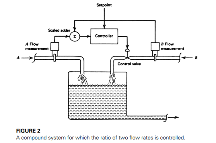
Compound Variable: In some cases, a single process-control loop is used to provide control of the relationship between two or more variables. This can be accomplished by using measurements from, say, two sensors as input to the process controller.

• A signal conditioning system must scale the two measurements and add them prior to input to the controller for evaluation and action. The analysis of such systems can become quite complicated.

• A common example is when the ratio of two reactants must be controlled. In this case, one of the flow rates is measured but allowed to float (that is, not regulated), and the other is both measured and adjusted to provide the specified constant ratio.

• An example of this system is shown in Figure. The flow rate of reactant A is measured and added, with appropriate scaling, to the measurement of flow rate B. The controller reacts to the resulting input signal by adjustment of the control valve in the reactant B input line.

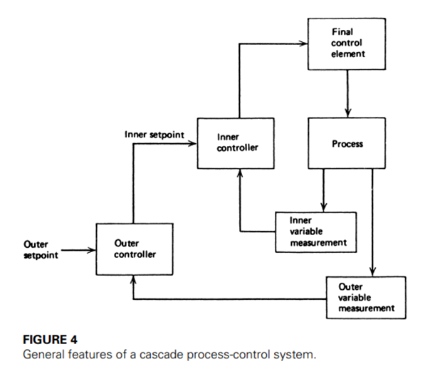
Cascade Control

• The inherent interaction that occurs between two control systems in many applications is sometimes used to provide better overall control. One method of accomplishing this is for the setpoint in one control loop to be determined by the measurement of a different variable for which the interaction exists.

• A block diagram of such a system is shown in Figure. Two measurements are taken from the system and each is used in its own control loop. In the outer loop, however, the controller output is the setpoint of the inner loop.

• Thus, if the outer loop controlled variable changes, the error signal that is Input to the controller effects a change in setpoint of the inner loop. Even though the measured value of the inner loop has not changed, the inner loop experiences an error signal, and thus new output by virtue of the setpoint change.

• Cascade control generally provides better control of the outer loo variable than is accomplished through a single-variable system.

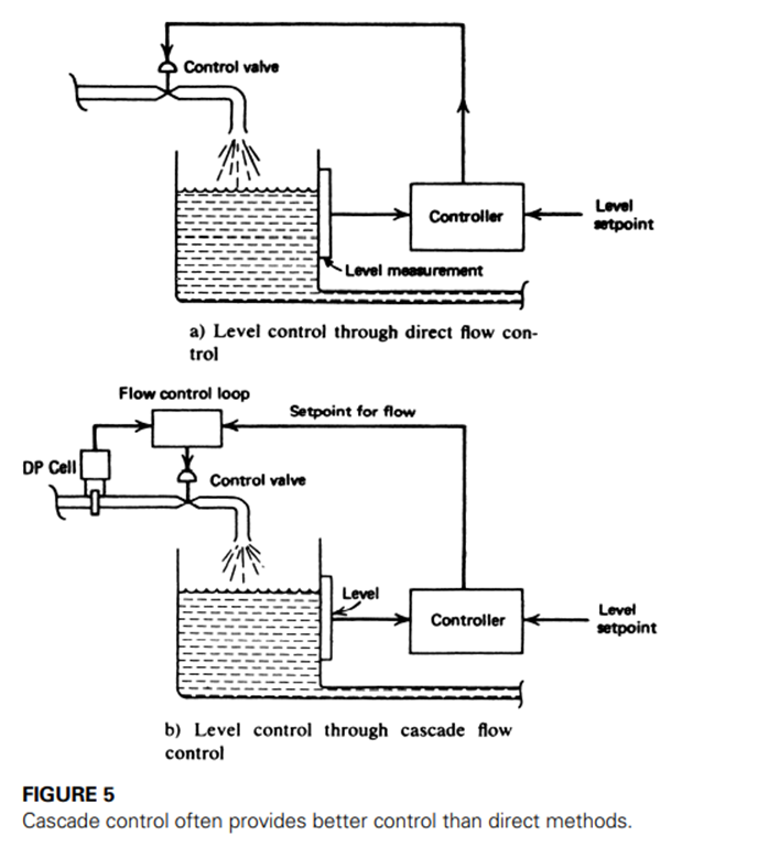
An example of a cascade control system not only shows how it works but suggests how control is improved. Consider the problem of controlling the level of liquid in a tank through regulation of the input flow rate. A single-variable system to accomplish this is shown in Figure a.

• A level measurement is used to adjust a flow-control valve as a final control element. The setpoint to the controller establishes the desired level. In this system, upstream load changes cause changes in flow rate that result in level changes. The level change is, however, a second-stage effect here. Consequently, the system cannot respond until the level has actually been changed by the flow rate change.

• Figure b shows the same control problem solved by a cascade system. The flow loop is a single-variable system as described earlier, but the setpoint is determined by a measurement of level. Upstream load changes never seen in the level of liquid in the tank because the flow-control system regulates such changes before they appear as substantial changes in level.

Multivariable control systems

➢One could correctly say that any reasonably complex industrial process is multivariable because many variables exist in the process and must be regulated. In general, however, many of these are either non interacting or the interaction is not a serious problem in maintaining the desired control functions.

➢In such cases, either single-variable controls or cascade loops suffice to effect satisfactory control of the overall process. The use of the word multivariable refers to those processes wherein many strongly interacting variables are involved.

➢Such a multivariable system can have such a complex interaction pattern that the adjustment of a single setpoint causes a profound influence on many other control loops in the process. In some cases, instabilities, cycling, or even runaway result from the indiscriminate adjustment of a few setpoints.

A) Analog Control

✓ When analog control loops are used in multivariable systems, a carefully prepared instructional set must be provided to the process personnel regarding the procedure for adjustment of setpoints. Generally, such adjustments are carried out in small increments to avoid instabilities that may result from large changes.

✓ Suppose we have a reaction vessel in which two reactants are mixed, react, and the product is drawn from the bottom. We are now concerned with controlling the reaction rate. It is also important, however, to keep the reaction temperature and vessel pressure below certain limits, and finally, the level is to be controlled at some nominal value.

✓ If the reactions are exothermic—that is, self-sustaining and heat-producing—then the relation among all of these parameters can be critical. If the temperature is low, then an indiscriminate increase in steam-flow setpoint could cause an unstable runaway of the reaction.

✓ Perhaps, in this case, the level and reaction flow rates must be altered as the steam-flow rate is increased to maintain control. The necessary steps are often empirically determined or from numerical solutions of complicated control equations.

B) Supervisory and Direct Digital Control

✓ The computer is ideally suited to the type of control problem presented by the multivariable control system. The computer can make any necessary adjustments of system operating points in an incremental fashion, according to a predetermined sequence, while monitoring process parameters for interactive effects.

✓ The problem in such a system is determining the algorithm that the computer must follow to provide the control function of the setpoint-change sequence. In some cases, control equations are used. Usually, in complex interactions, these relations are not analytically known.

✓ In some cases, self-adapting algorithms are used, causing the computer to sequence through a set of operations and letting the result of one operation determine the next operation. As an example, if the temperature is slightly raised and the pressure rises, then drop the temperature, and so on.

✓ The computer can sequence through a myriad of such micro-adjustments of setpoints looking for the optimum adjustment path.

Stability

Transfer Function Frequency Dependence:

▪The static transfer function of an element in a process-control loop tells how the output is determined fromthe input when the input is constant in time.

▪The dynamic transfer function of an element tells how the output is determined from the input when theinput varies in time.

▪For the study of stability, we are interested in the particular time variation that is sinusoidal (i.e., the dynamic transfer function when the input is oscillating at some frequency, f ).

Consider some element block as shown in Figure with a transfer function, T(ω), and where the input is a sinusoidal given by; r = a sin(ω t)

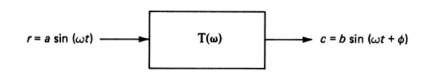
A transfer function changes the amplitude and phase of a sinusoidal input

The frequency has been expressed in terms of the angular frequency ω = 2πf measured in radians/second. There are only two things that can happen, in a linear study at least: The amplitude can change, and there can be a phase shift. Thus, the output can be described as;

c = b sin(ω t + φ)

The ratio of the amplitudes is called the gain; gain=b/a , and the phase shift is called the phase lag, φ. In general, both the gain and amount of phase lag of an element vary with frequency. The gain decreases, and the phase lag becomes larger. The whole issue of stability is tied up with the frequency variation of gain and phase of all elements in a control loop.

Source of Instability: To see how a process-control loop can cause instability, consider the open-loop block diagram of

Figure, for which an oscillating transient disturbance has been imposed at r. Notice that the feedback line has been broken at the error detector, so no actual feedback occurs. Each element of the loop has a gain and phase lag, including the process itself. The net gain is the product of all gains, and the net phase lag is the sum of all phase lags.

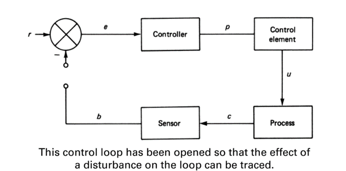
In a perfect world, the feedback, b, would be an exact replica of the disturbance at every frequency. This would mean a loop gain of unity and no phase shift. Then the phase shift (lag) of the error detector would subtract the feedback from the disturbance, and it would be cancelled. In reality, there are gain variations and extra phase shifts, and both vary with the disturbance frequency.

As the gain becomes smaller with frequency, the effectiveness of the feedback to cancel error is reduced. But the control system is still working and stable.

Stability Criteria

• We can derive stability criteria by determining just what conditions of system gain and phase lag can lead to an enhancement of error. We are led to two conclusions:

1. The gain must be greater than 1.

2. The phase shift must be -180 degrees (lag).

• Thus, if there is any frequency for which the gain is greater than one and the phase is -180 degrees, the system is unstable. From this argument, we develop two ways of specifying when a system is stable. These rules are as follows:

➢ Rule 1: A system is stable if the phase lag is more positive than -180 degrees at the frequency for which the gain is unity (one).

➢ Rule 2: A system is stable if the gain is less than one (unity) at the frequency for which the phase lag is -180 degrees.

• The application of these rules to an actual process requires evaluation of the gain and phase shift of the system for allfrequencies to see if Rules 1 and 2 are satisfied. This is easier to do if a plot of gain and phase versus frequency is used (Bode Plot).

Process loop tuning.

➢The last aspect of process-control technology we consider refers to the actual start-up and adjustment of a process-control loop.

➢We have seen how the various settings of the controller can have a profound effect on loop performance. Now, themost natural question is how to select these settings.

➢There are, in fact, many methods for determination of the optimum mode gains, depending on the nature and complexity of the process. We consider here three common tuning methods to give a basic idea of how optimum adjustments are found.

➢Two of the methods given are semi-empirical in that they depend on measurements made on the system to determine factors used in the adjustment formulas.

Open-Loop Transient Response Method

▪This method of finding controller settings was developed by Ziegler and Nichols and is sometimes referred to as a process-reaction method. The basic approach is to open the process control loop so that no control action (feedback) occurs. This usually is done by disconnecting the controller output from the final control element. All of the process parameters are held at their nominal values. This method can be used only for systems with self-regulation.

At some time, a transient disturbance is introduced by a small, manual change of the controlling variable using the final control elements. This change should be as small as practical for making necessary measurements. The controlled variable is measured (recorded) versus time at the instant of and following the disturbance.

Open-Loop Transient Response Method

A typical open-loop controller response is shown in Figure , where the disturbance is applied at t₁

We have expressed the deviation as a percent of range as usual, and we assume the final control element disturbance also is expressed as a percentage change.

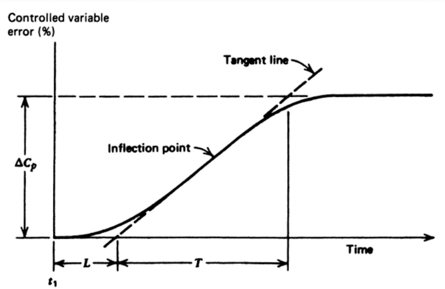
• A tangent line, shown as a dashed line, is drawn at the inflection point of the curve. The inflection point is defined as that point on the curve where the slope stops increasing and begins to decrease. Where the tangent line crosses the origin, we get

L = lag time in minutes

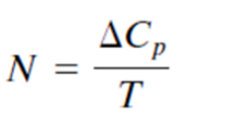
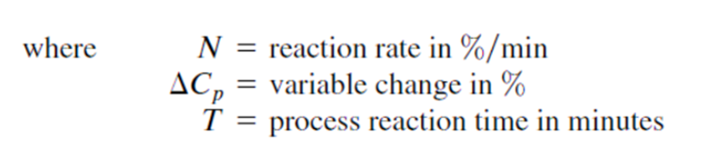
as the time from disturbance application to the tangent line intersection as shown in Figure. Also from the graph we get T, the process reaction time, and

The following paragraphs give the stable control definitions for the various modes as developed by Ziegler and Nichols and corrections developed by Cohen and Coon (when the quarter-amplitude response criterion is indicated). In the latter

case, a log ratio is used, defined by

where R = log ratio (unitless)