Images sensing and Acquisition:

There are 3 principal sensor arrangements (produce an electrical output proportional to light intensity).

(i)Single imaging Sensor (ii)Linesensor (iii)Array sensor

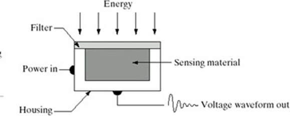
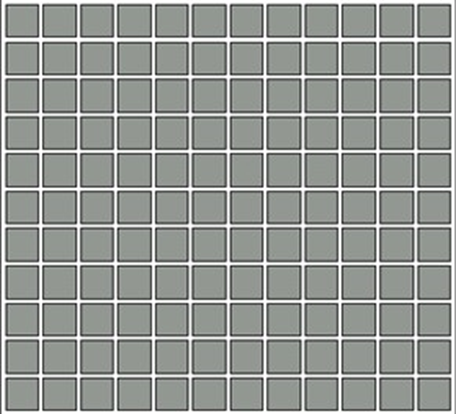
Image Acquisition using a single sensor

The most common sensor of this type is the photodiode, which is constructed of silicon materials and whose output voltage waveform is proportional to light. The use of a filter in front of a sensor improves selectivity. For example, a green (pass) filter in front of a light sensor favours light in the green band of the color spectrum. As a consequence, the sensor output will be strongerfor green light than for other componentsin the visible spectrum.

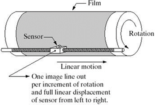
Fig: Combining a single sensor with motion to generate a 2-Dimage

In order to generate a 2-D image using a single sensor, there have to be relative displacements in both the x- and y-directions between the sensor and the area to be imaged. An arrangement usedin high precision scanning, where a film negative is mounted onto a drum whose mechanical rotation provides displacement in one dimension. The single sensor is mounted on a lead screw that provides motion in the perpendicular direction. Since mechanical motion can be controlled with high precision, this method is an inexpensive (but slow) way to obtain high-resolution images.

Image Acquisition using Sensor Strips

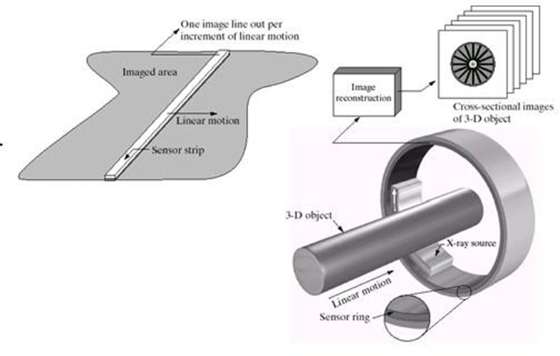
Fig: (a) Image acquisition using linear sensor strip (b) Image acquisition usingcircular sensor strip.

The strip provides imaging elements in one direction. Motion perpendicular to the strip provides imaging in the other direction. This is the type of arrangement used in most flatbed scanners. Sensing devices with 4000 or more in-line sensors are possible. In-line sensors are used routinely in airborne imaging applications, in which the imaging system is mounted on an aircraft that flies at a constant altitude and speed over the geographical area to be imaged. One-dimensional imaging sensor strips that respond to various bands of the electromagnetic spectrum are mounted perpendicular to the direction of flight. The imaging strip gives one line of an image at a time, and the motion of the strip completes the other dimension of a two-dimensional image. Sensor strips mounted in a ring configuration are used in medical and industrial imaging to obtain cross- sectional (“slice”) images of 3-D objects. A rotating X-ray source provides illumination and the portion of the sensorsopposite the source collect the X-ray energy that pass through the object  (the sensors obviously have to be sensitive to X ray energy). This is the basis for medical and industrial computerized axial tomography (CAT) imaging.

Image Acquisition using Sensor Arrays

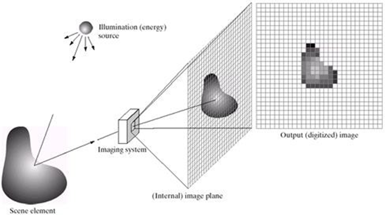
Fig: An example of the digitalimage acquisition process(a) energy source (b) Anelement of a scene (d) Projection of the scene into the image (e) digitized image

This type of arrangement is found in digital cameras. A typical sensor for these cameras is a CCD array, which can be manufactured with a broad range of sensing properties and can be packaged in rugged arrays of 4000 * 4000 elements or more. CCD sensors are used widely in digitalcameras and other light sensinginstruments. The responseof each sensor is proportional to the integral of the light energy projected onto the surface of the sensor, a property that is used in astronomical and other applications requiring low noiseimages.

The first function performed by the imaging system is to collect the incoming energy and focus it onto an image plane. If the illumination is light, the front end of the imaging system is a lens, which projects the viewed scene onto the lens focal plane. The sensor array, which is coincident with the focal plane, produces outputs proportional to the integral of the light received at each sensor.

Images sampling and Quantization’s

In Digital Image Processing, signals captured from the physical world need to be translated into digital form by “Digitization” Process. In order to become suitable for digital processing, an image function f(x,y) must be digitized both spatially and in amplitude. This digitization process involves two main processes called

1. Sampling: Digitizing the co-ordinate value is called sampling.

2. Quantization: Digitizing the amplitude value is called quantization

Typically, a frame grabber or digitizer is used to sample and quantize the analogue video signal.

Sampling

Since an analogue image is continuous not just in its co-ordinates (x axis), but also in its amplitude (y axis), so the part that deals with the digitizing of co-ordinates is known as sampling. In digitizing sampling is done on independent variable. In case of equation y = sin(x), it is done on x variable.

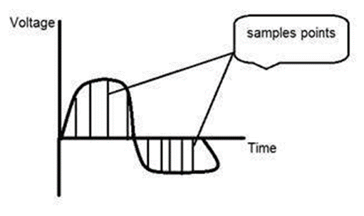
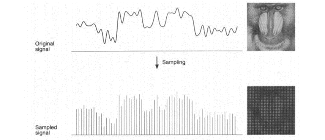
When looking at this image, we can see there are some random variations in the signal caused by noise. In sampling we reduce this noise by taking samples. It is obvious that more samples we take, the quality of the image would be more better, the noise would be more removed and same happens vice versa. However, if you take sampling on the x axis, the signal is not converted to digital format, unless you take sampling of the y-axis too which is known as quantization.

Sampling has a relationship with image pixels. The total number of pixels in an image can be calculated as Pixels = total no of rows * total no of columns. For example, let’s say we have total of 36 pixels, that means we have a square image of 6X 6. As we know in sampling, that more samples eventually result in more pixels. So it means that of our continuous signal, we have taken 36 samples on x axis. That refers to 36 pixels of this image. Also the number sample is directly equal to the number of sensors on CCD array.

Here is an example for image sampling and how it can be represented using a graph.

Quantization

Quantization is opposite to sampling because it is done on “y axis” while sampling is done on “x axis”. Quantization is a process of transforming a real valued sampled image to one taking only a finite number of distinct values. Under quantization process the amplitude values of the image are digitized. In simple words, when you are quantizing an image, you are actually dividing a signal into quanta(partitions).

Now let’s see how quantization is done. Here we assign levels to the values generated by sampling process. In the image showed in sampling explanation, although the samples has been taken, but they were still spanning vertically to a continuous range of gray level values. In the image shown below, these vertically ranging values have been quantized into 5 different levels or partitions. Ranging from 0 black to 4 white. This level could vary according to the type of image you want.

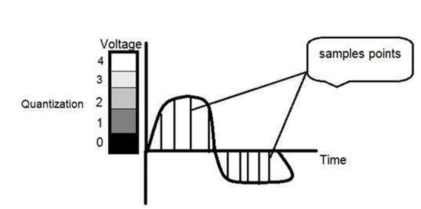
There is a relationship between Quantization with gray level resolution. The above quantized image represents 5 different levels of gray and that means the image formed from this signal, would only have 5 different colors. It would be a black and white image more or less with some colors of gray.

When we want to improve the quality of image, we can increase the levels assign to the sampled image. If we increase this level to 256, it means we have a gray scale image. Whatever the level which we assign is called as the gray level. Most digital IP devices uses quantization into k equal intervals. If b-bits per pixel are used,

Spatial and Gray-Level Resolution

Spatial resolution is the smallestdiscernable (detect with difficulty )changein an image. Gray- levelresolution is the smallestdiscernable (detect with difficulty) change in gray level.

Image resolution quantifies how much close two lines (say one dark and one light) can be to each other and still be visibly resolved. The resolution can be specified as number of lines per unit distance, say 10 lines per mm or 5 line pairs per mm. Another measure ofimage resolution is dots per inch, i.e. the number of discernible dots per inch.

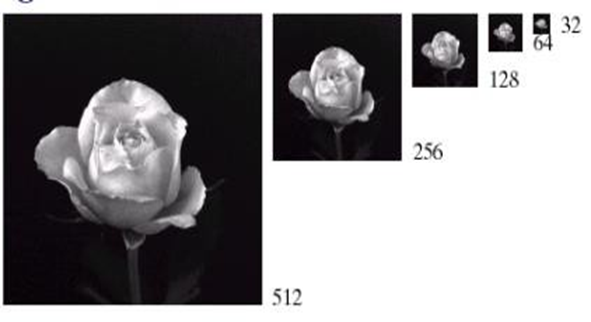
Fig: A 1024 x 2014,8 bit image subsampled down to size32 x 32 pixels. The numberof allowable kept at 256.

Image of size 1024*1024 pixels whose gray levels are represented by 8 bits is as shown in fig above. The results of subsampling the 1024*1024 image. The subsampling was accomplished by deleting the appropriate number of rows and columns from the original image. For example, the 512*512 image was obtained by deleting every other row and column from the 1024*1024 image. The 256*256image was generated by deleting every other row and column in the 512*512 image, and so on. The number of allowed gray levels was kept at 256. These images show dimensional proportions between various sampling densities, but their size differences make it difficult to see the effects resulting from a reduction in the number of samples. The simplest way to compare these effects is to bring all the subsampled images up to size 1024 x 1024.

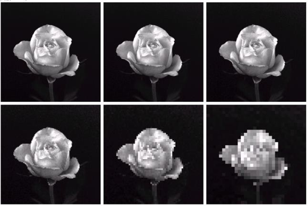
Fig: (a) 1024 x 1024, 8 bit image (b) 512 x 512 image resampled into 1024 x 1024 pixels by row and column duplication. (c) through (f) 256 x 256, 128 x 128, 64 x 64, and 32 x 32 images resampled into 1024 x 1024 pixels.

Gray-Level Resolution

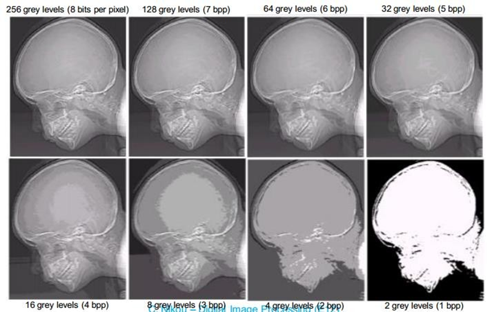
Fig: 452 x 374, 256 level image. (b)- (d) Image displayed in 128, 64, 32,16,8,4 and 2 grey level, while keeping spatial resolution constant.

In this example, we keep the number of samples constant and reduce the number of grey levels from 256 to 2.

Aliasing and Moire Patterns

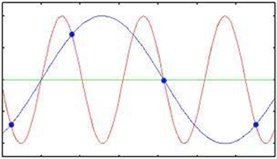
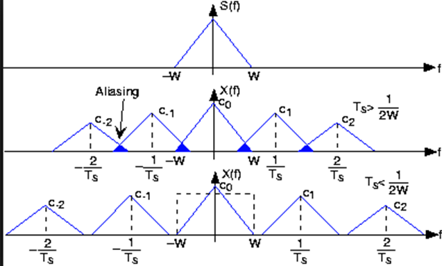
Shannon sampling theorem tells us that, if the function is sampled at a rate equal to or greater than twice its higest frequency(f_s≥f_m )it is possible to recover completely the original function from the samples. If the functionis undersampled, then a phenonmemnon called alising(distortion) (If two pattern or spectrum overlap, the overlapped portion is called aliased) corrupts the sampled image. The corruption is in the form of additional frequency components being introduced into the sampled function. These are called aliased frequencies.

The principal approach for reducing the aliasing effects on an image is to reduce its high- frequency components by blurring the image prior to sampling. However, aliasing is always present in a sampled image. The effect of aliased frequencies can be seen under the right conditions in the form of so called Moiré patterns.

A moiré pattern is a secondary and visually evident superimposed pattern created, for example, when two identical (usually transparent) patterns on a flat or curved surface (such as closely spaced straight lines drawn radiating from a point or taking the form of a grid) are overlaid while displaced or rotated a small amountfrom one another.

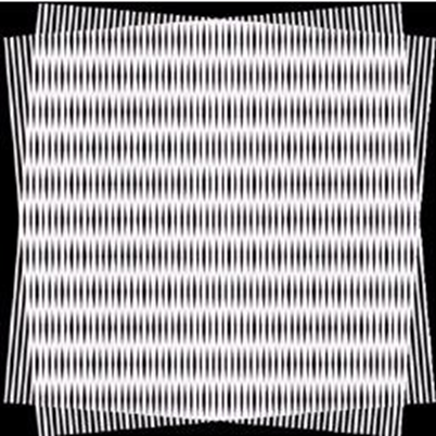
Fig: Illustration of the moire effect

Zooming and Shrinking Digital Image

Zooming may be viewed as oversampling and shrinking many be viewed as undersampling.

Zooming is a method of increasing the size of a given image. Zooming requires two steps: creation of new pixel locations, and the assigningnew grey level values to those new locations

Nearest neighbor interpolation: Nearest neighbor interpolation is the simplest method and basically makes the pixels bigger. The intensity of a pixel in the new image is the intensity of the nearestpixel of the original image. If you enlarge 200%, one pixel will be enlarged to a 2 x 2 area of4 pixels with the same color as the original pixel.

Bilinear interpolation: Bilinear interpolation considers the closest 2x2 neighborhood of known pixel values surrounding the unknown pixel. It then takes a weighted average of these 4 pixels to arrive at its final interpolated value. This results in much smoother looking images than nearest neighbour.

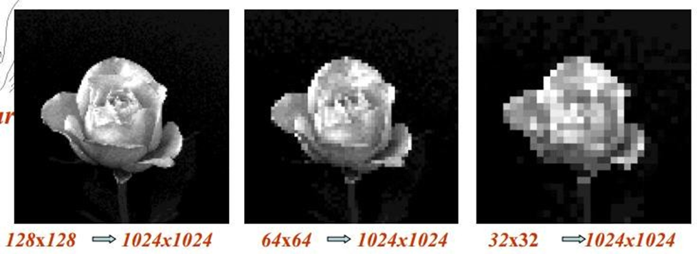
Fig: Images zoomed from 128 x 128, 64 x 64 and 32 x 32 pixelsto 1024 x 1024 pixels usingnearest neighbor grey-level interpolation.

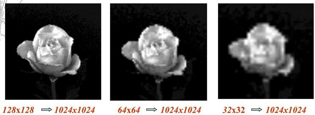
Fig: Images zoomed from 128 x 128, 64 x 64 and 32 x 32 pixels to 1024 x 1024 pixelsusing bilinear interpolation.

Image shrinking is done in a similar manner as just described for zooming. The equivalent process of pixel replication is row-column deletion. For example, to shrink an image by one-half, we delete every other row and column.

Some Basic Relationships between Pixels

(Note- Sums involved see youtube)

An image is denoted by f (x, y). When referring in this section to a particular pixel, we use lowercase letters, such as p and q.

Neighbors of a Pixel

A pixel p at coordinates (x, y) has four horizontal and vertical neighbors whose coordinates are given by

(x +1, y), (x -1),y), (x, y + 1), (x, y – 1)

And are denoted by N_D(P). These points together with the 4 neighbors, are called the 8- neighbors of p, denoted by N₈(P)_. As before some of the neighbour locations in N_D(P). and N₈(P). fall outside the image if (x, y) is on the border of the image.

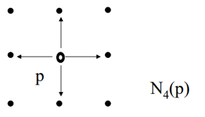
4-neighbors of a pixel p are its vertical and horizontal neighbors denoted by N₄(p)

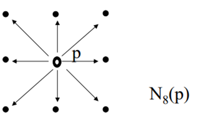
8-neighbors of a pixel p are its vertical horizontal and 4 diagonal neighbors denoted by N₈(p)

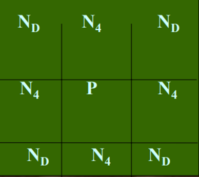
•N 4 - 4-neighbors

•N D - diagonal neighbors

•N 8 - 8-neighbors (N 4 U N D )

Adjacency

• Two pixels are connected if they are neighbors and their gray levels satisfy some specified criterion of similarity.

• For example, in a binary image two pixels are connected if they are 4-neighbors and have same value (0/1)

Let V be set of gray levels values used to define adjacency.

• 4-adjacency: Two pixels p and q with values from V are 4- adjacent if q is in the set N 4 (p).

• 8-adjacency: Two pixels p and q with values from V are 8- adjacent if q is in the set N 8 (p).

• m-adjacency: Two pixels p and q with values from V are m-adjacent if,

– q is in N₄(P).

Types of adjacency

1. 4-adjacency: Two pixels p and q with values from v are 4-adjacent if q is in the set N₄ (p).

2. 8-adjacency: Two pixels p and q with values from v are 8-adjacent if q is in the set N₈ (p).

3. m-adjacency (mixed): two pixels p and q with values from v are m-adjacent if:

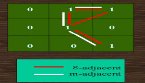
• Mixed adjacency is a modification of 8-adjacency ''introduced to eliminate the ambiguities that often arise when 8- adjacency is used. (eliminate multiple path connection)

• Pixel arrangement as shown in figure for v= {1}

Path

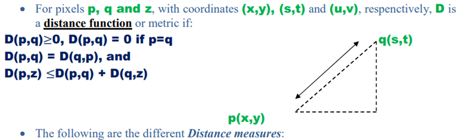
• A digital path (or curve) from pixel p with coordinate (x,y) to pixel q with coordinate (s,t) is a sequence of distinct pixels with coordinates (x₀ , y₀ ), (x₁ , y₁ ), ..., (x_n , y_n ), where (x₀ , y₀ )= (x,y), (x_n , y_n )= (s,t)

• (x_i , y_i ) is adjacent pixel (x_i-1, y_i-1) for 1≤j≤n ,

• n- The length of the path.

• If (x₀ , y₀ )= (x_n , y_n):the path is closed path.

• We can define 4- ,8- , or m-paths depending on the type of adjacency specified.

Connectivity

• Let S represent a subset of pixels in an image, Two pixels p and q are said to be connected in S if there exists a path between them.

• Two image subsets S1 and S2 are adjacent if some pixel in S1 is adjacent to some pixel in S2

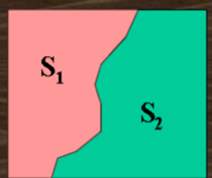
Region

• Let R to be a subset of pixels in an image, we call a R a region of the image. If R is a connected set.

• Region that are not adjacent are said to be disjoint.

• Example: the two regions (of Is) in figure, are adjacent only if 8-adjacany is used.

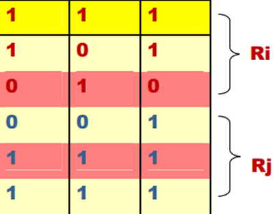
4-path between the two regions does not exist, (so their union in not a connected set).

• Boundary (border) image contains K disjoint regions, R_k , k=1, 2, ...., k, none of which touches the image border

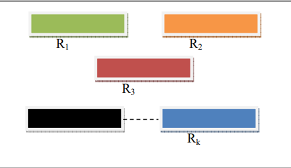
• Let: Ru - denote the union of all the K regions, (R_u)^c- denote its complement of a set S is the set of points that are not in s).

(R_u)^c - called background of the image. Boundary (border or contour) of a region R is the set of points that are adjacent to of R (another way: the border of a region is the set of pixels in the reigion that have at least are background neighbour).

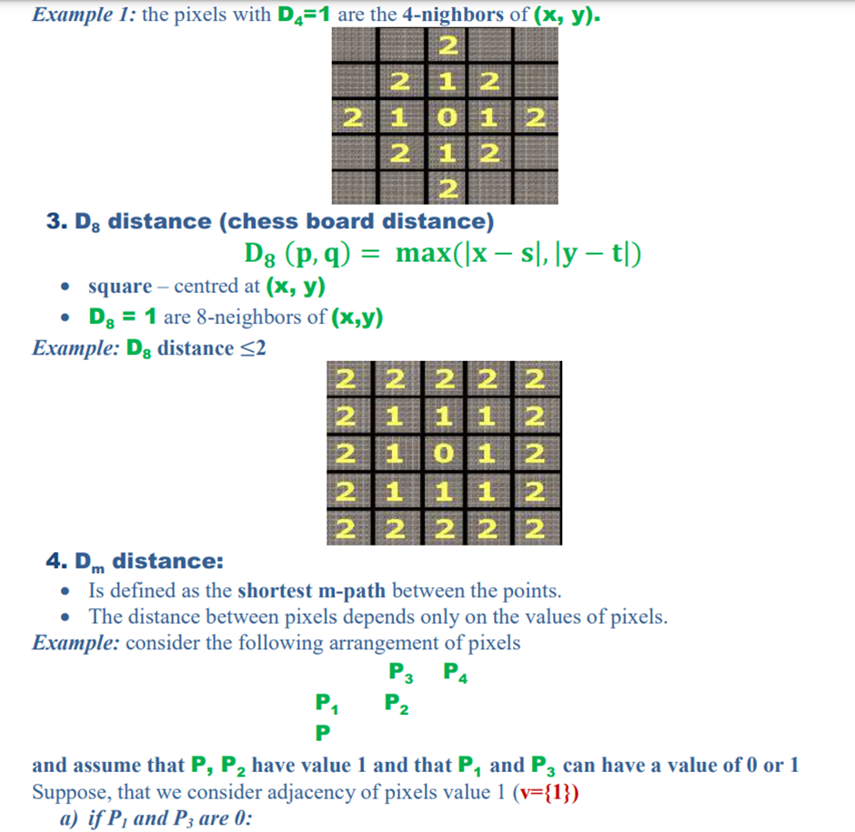
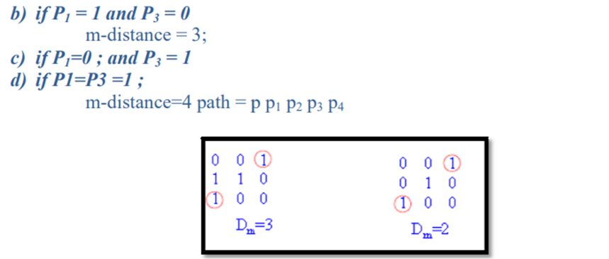
Distance Measures

Difference between image sampling and Quantzaition

Linear and Nonlinear Operations.

H(af+bh)=aH(f)+bH(g)

• Where H is an operator whose input and outputare images.

• f and g are two images

• a and b are constants.

H is said to belinear operation if it satisfiesthe above equationor else H is a nonlinear operator.