
Digital Image Processing 4th Module
IMAGE ENHANCEMENT IN THE SPATIAL DOMAIN
Image enhancement approaches fall into two broad categories: spatial domain methods and frequency domain methods. The term spatial domain refers to the image plane itself, and approaches in this category are based on direct manipulation of pixels in an image. Frequency domain processing techniques are based on modifying the Fourier transform of an image.
The term spatial domain refers to the aggregate of pixels composing an image. Spatial domain methods are procedures that operate directly on these pixels. Spatial domain processes will be denoted by the expression
g (x, y) = T [f (x, y)]
where f(x, y) is the input image, g(x, y) is the processed image, and T is an operator on f, defined over some neighborhood of (x, y). In addition, T can operate on a set of input images, such as performing the pixel-by-pixel sum of K images for noise reduction.
The principal approach in defining a neighborhood about a point (x, y) is to use a square or rectangular sub image area centered at (x, y), as shown in below figure 1.
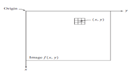
The center of the sub image is moved from pixel to pixel starting, say, at the top left corner. The operator T is applied at each location (x, y) to yield the output, g, at that location. The process utilizes only the pixels in the area of the image spanned by the neighborhood. Although other neighborhood shapes, such as approximations to a circle, sometimes are used, square and rectangular arrays are by far the most predominant because of their ease of implementation.
The simplest form of T is when the neighborhood is of size 1*1 (that is, a single pixel). In this case, g depends only on the value of f at (x, y), and T becomes a gray-level (also called an intensity or mapping) transformation function of the form s = T(r) where, for simplicity in notation, r and s are variables denoting, respectively, the gray level of f(x, y) and g(x, y) at any point (x, y).
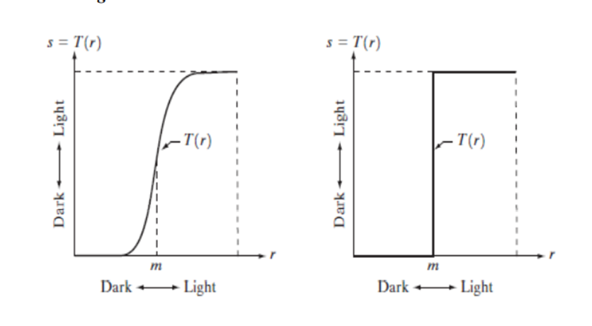
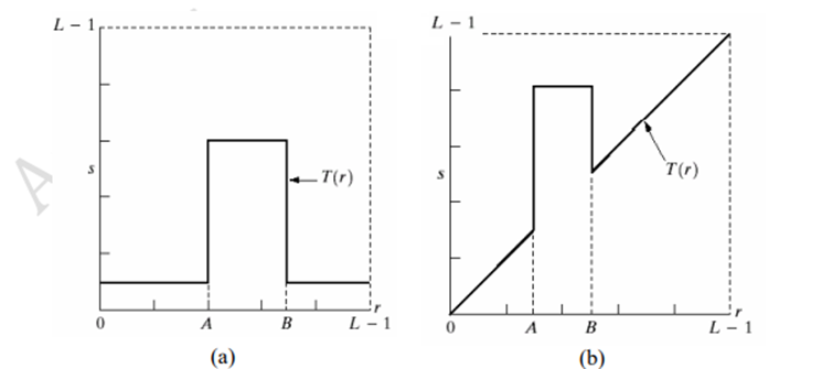
For example, if T(r) has the form shown in Fig. 2(a), the effect of this transformation would be to produce an image of higher contrast than the original by darkening the levels below m and brightening the levels above m in the original image.
In this technique, known as contrast stretching, the values of r below m are compressed by the transformation function into a narrow range of s, toward black. The opposite effect takes place for values of r above m. In the limiting case shown in Fig. 2(b), T(r) produces a two-level (binary) image. A mapping of this form is called a thresholding function.
Some Basic Gray Level Transformations (Intensity Transformation)
1. Image Negatives:
The negative of an image with gray levels in the range [0,L-1]is obtained by using the negative transformation shown in Fig. 3.3, which is given by the expression
s = L - 1 – r
Reversing the intensity levels of an image produces the equivalent of a photographic negative. This type of processing is particularly suited for enhancing white or gray detail embedded in dark regions of an image, especially when the black areas are dominant in size.
2. Log Transformations: The general form of the log transformation
s = c log (1 + r)
where c is a constant, and it is assumed that r ≥ 0.
The shape of the log curve in Fig. 3 shows that this transformation maps a narrow range of low gray-level values in the input image into a wider range of output levels. The opposite is true of higher values of input levels. We would use a transformation of this type to expand the values of dark pixels in an image while compressing the higher-level values. The opposite is true of the inverse log transformation.
3. Power-Law Transformations
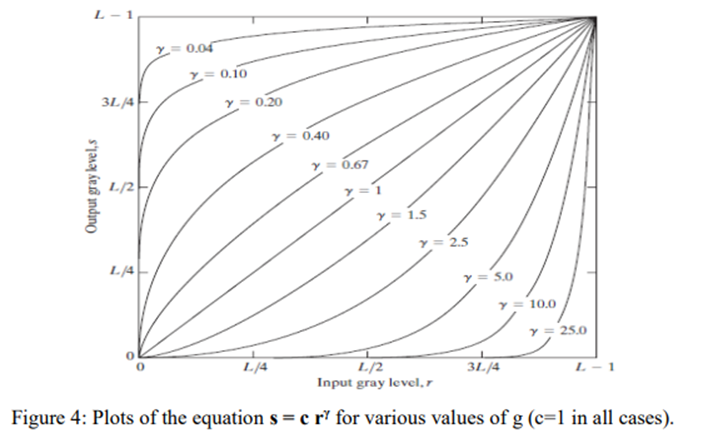
Power-law transformations have the basic form
s = c rγ
where c and γ are positive constants, Also can be represented as
s = c (r+ε)γ
An offset measurable when input is zero
We see in Fig. 4 that curves generated with values of g>1 have exactly the opposite effect as those generated with values of g<1. Finally, we note that from above equation reduces to the identity transformation when c=g=1
Plots of s versus r for various values of g are shown in Fig. 4. As in the case of the log transformation, power-law curves with fractional values of g map a narrow range of dark input values into a wider range of output values, with the opposite being true for higher values of input levels.
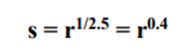
A variety of devices used for image capture, printing, and display respond according to a power law. By convention, the exponent in the power-law equation is referred to as gamma. The process used to correct this power-law response phenomenon is called gamma correction. Gamma correction is straightforward. All we need to do is preprocess the input image before inputting it into the monitor by performing the transformation
Gamma correction is important if displaying an image accurately on a computer screen is of concern. Images that are not corrected properly can look either bleached out, or, what is more likely, too dark.
For example, cathode ray tube (CRT) devices have an intensity-to-voltage response that is a power function, with exponents varying from approximately 1.8 to 2.5.With reference to the curve for g=2.5 in Fig. 3.6, we see that such display systems would tend to produce images that are darker than intended.
Piecewise-Linear Transformation Functions: Piece-wise Linear Transformation is type of gray level transformation that is used for image enhancement. It is a spatial domain method. It is used for manipulation of an image so that the result is more suitable than the original for a specific application.
Some commonly used piece-wise linear transformations are:
Contrast stretching
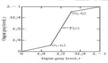
One of the simplest piecewise linear functions is a contrast-stretching transformation. Low-contrast images can result from poor illumination, lack of dynamic range in the imaging sensor, or even wrong setting of a lens aperture during image acquisition. The idea behind contrast stretching is to increase the dynamic range of the gray levels in the image being processed.
· If r1,s1 and r2,s2 control the shape of the transformation function.and if r1=s1 and r2=s2 the transformation is a linear function that produces no changes in intensity levels
· If r1=r2 and s1=0 and s2 =L-1, the transformation becomes a thresholding function that creates a binary image.
· In general r1≤r2 and s1 ≤s2 is assumed so that the function is single valued and monotonically increasing. This preserves the order of intensity levels, thus preventing the creation of intensity artifacts in the processed image.
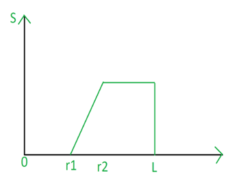
Clipping:
A special case of contrast stretching is clipping where l=n=0. It is used for noise reduction when the input signal is known. It puts all grey levels below r1 to black(0) and above r2 to white(1).
Thresholding:
Another special case of contrast stretching is thresholding where l=m=t. It is also used for noise reduction. It preserves the grey levels beyond r1.
Gray level slicing
It is highlighting a specific range of intensities in an image often is of interest. Its applications include enhancing features such as masses of water in satellite imagery and enhancing flaws in X-ray images. · The intensity level slicing process can be implemented for these defects/noise etc.
· It can be done in several ways
Ex: One is to display in one value (say, white), all the values in the range of interest and in another (say, black), all other intensities.
Bit-plane slicing
Instead of highlighting gray-level ranges, highlighting the contribution made to total image appearance by specific bits might be desired. Suppose that each pixel in an image is represented by 8 bits. Imagine that the image is composed of eight 1-bit planes, ranging from bit-plane 0 for the least significant bit to bit plane 7 for the most significant bit. In terms of 8-bit bytes, plane 0 contains all the lowest order bits in the bytes comprising the pixels in the image and plane 7 contains all the high-order bits.
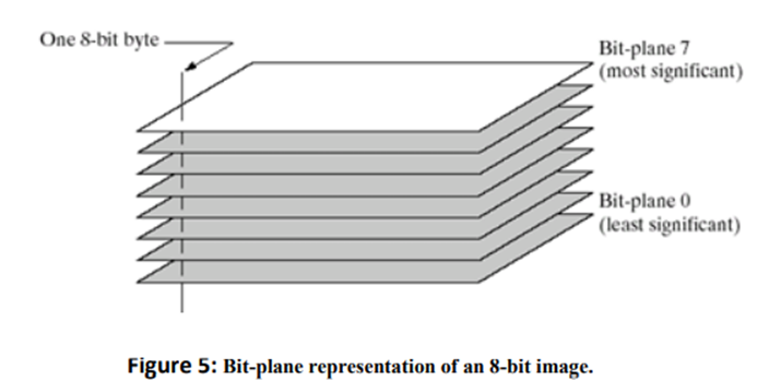
Decomposing an image into its bit planes is useful for analyzing the relative importance of each bit in the image, a process that aids in determining the adequacy of the number of bits used to quantize the image. It is useful in image compression.
· The reconstruction is done by using few planes only.
· It is done by multiplying the pixels of the nth plane by a constant 2n-1 .
· All the generated planes are added together (few of 8 planes)
· If we use bit plane 7 and 8, multiply bit plane 8 by 128 and plane 7 by 64 and then added together.
Histograph processing (sums)
Enhancement Using Arithmetic/Logic Operations
Arithmetic/logic operations involving images are performed on a pixel-by-pixel basis between two or more images (this excludes the logic operation NOT, which is performed on a single image). Logic operations similarly operate on a pixel-by-pixel basis. We need only be concerned with the ability to implement the AND, OR, and NOT logic operators because these three operators are functionally complete.
When dealing with logic operations on gray-scale images, pixel values are processed as strings of binary numbers. For example, performing the NOT operation on a black, 8-bit pixel (a string of eight 0’s) produces a white pixel (a string of eight 1’s).
Intermediate values are processed the same way, changing all 1’s to 0’s and vice versa. The four arithmetic operations, subtraction and addition (in that order) are the most useful for image enhancement.
Image Subtraction: The difference between two images f(x, y) and h(x, y), expressed as
g(x, y) = f(x, y) - h(x, y),
And it is obtained by computing the difference between all pairs of corresponding pixels from f and h. The key usefulness of subtraction is the enhancement of differences between images.
One of the most commercially successful and beneficial uses of image subtraction is in the area of medical imaging called mask mode radiography.
In this case h(x, y), the mask, is an X-ray image of a region of a patient’s body captured by an intensified TV camera (instead of traditional X-ray film) located opposite an X-ray source.
The procedure consists of injecting a contrast medium into the patient’s bloodstream, taking a series of images of the same anatomical region as h(x, y), and subtracting this mask from the series of incoming images after injection of the contrast medium. The net effect of subtracting the mask from each sample in the incoming stream of TV images is that the areas that are different between f(x, y) and h(x, y) appear in the output image as enhanced detail.
Image Averaging:
Consider a noisy image g(x, y) formed by the addition of noise h(x, y) to an original image f(x, y); that is,
g(x, y) = f(x, y) + h(x, y)
where the assumption is that at every pair of coordinates (x, y) the noise is uncorrelated and has zero average value. The objective of the following procedure is to reduce the noise content by adding a set of noisy images, {gi(x, y)}.
If the noise satisfies the constraints just stated, it can be shown that if an image
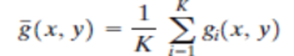
is formed by averaging K different noisy images,

An important application of image averaging is in the field of astronomy, where imaging with very low light levels is routine, causing sensor noise frequently to render single images virtually useless for analysis.
Multiplication and Division: We consider division of two images simply as multiplication of one image by the reciprocal of the other. Aside from the obvious operation of multiplying an image by a constant to increase its average gray level, image multiplication finds use in enhancement primarily as a masking operation that is more general than the logical masks discussed in the previous paragraph. In other words, multiplication of one image by another can be used to implement gray-level, rather than binary, masks.
Basics of Spatial Filtering:
Some neighborhood operations work with the values of the image pixels in the neighborhood and the corresponding values of a sub image that has the same dimensions as the neighborhood. The sub image is called a filter, mask, kernel, template, or window, with the first three terms being the most prevalent terminology. The values in a filter sub image are referred to as coefficients, rather than pixels.
The mechanics of spatial filtering are illustrated in Fig 8.The process consists simply of moving the filter mask from point to point in an image. At each point (x, y), the response of the filter at that point is calculated using a predefined relationship. For linear spatial, the response is given by a sum of products of the filter coefficients and the corresponding image pixels in the area spanned by the filter mask.
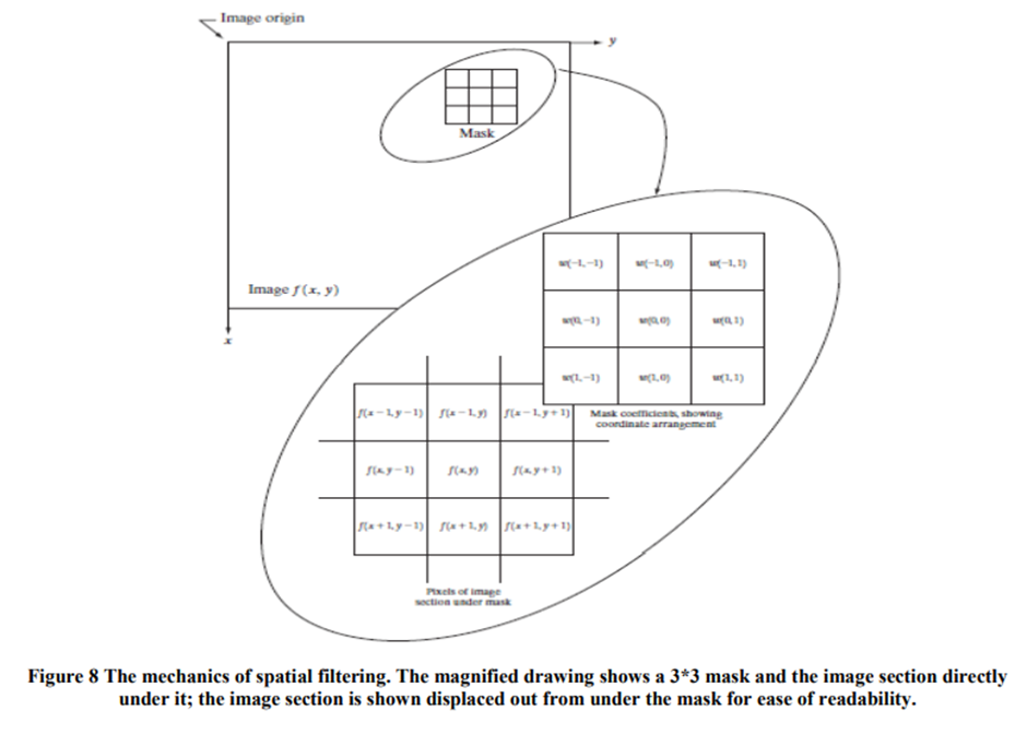
For the 3*3 mask shown in Fig. 3.32, the result (or response), R, of linear filtering with the filter mask at a point (x, y) in the image is
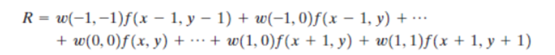
which we see is the sum of products of the mask coefficients with the corresponding pixels directly under the mask. Note in particular that the coefficient w(0, 0) coincides with image value f(x, y), indicating that the mask is centered at (x, y) when the computation of the sum of products takes place. For a mask of size m*n, we assume that m=2a+1 and n=2b+1,where a and b are nonnegative integers.
All this says is that our focus in the following discussion will be on masks of odd sizes, with the smallest meaningful size being 3*3 (we exclude from our discussion the trivial case of a 1*1 mask). In general, linear filtering of an image f of size M*Nwith a filter mask of size m*n is given by the expression:
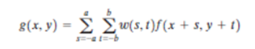
where, from the previous paragraph, a=(m-1)/2 and b=(n-1)/2. To generate a complete filtered image this equation must be applied for x=0, 1, 2, p , M-1 and y=0, 1, 2, p , N-1. When interest lies on the response, R, of an m*n mask at any point (x, y), and not on the mechanics of implementing mask convolution, it is common practice to simplify the notation by using the following expression:
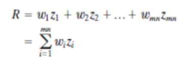
where the w’s are mask coefficients, the z’s are the values of the image gray levels corresponding to those coefficients, and mn is the total number of coefficients in the mask.
Image enhancement in the Frequency Domain
The frequency domain methods of image enhancement are based on convolution theorem. This is represented as,
g(x, y) = h (x, y)*f(x, y)
Where. g(x, y) = Resultant image
h(x, y) = Position invariant operator
f(x, y)= Input image
The Fourier transform representation of the equation above is,
G (u, v) = H (u, v) F (u, v)
The function H (u, v) in equation is called transfer function. It is used to boost the edges of input image f (x, y) to emphasize the high frequency components.
The different frequency domain methods for image enhancement are as follows. 1. Contrast stretching. 2. Clipping and thresholding. 3. Digital negative. 4. Intensity level slicing and 5. Bit extraction.
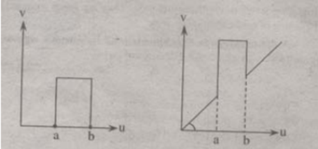
1. Contrast Stretching: Due to non-uniform lighting conditions, there may be poor contrast between the background and the feature of interest. Figure 1.1 (a) shows the contrast stretching transformations.
In the area of stretching the slope of transformation is considered to be greater than unity. The parameters of stretching transformations i.e., a and b can be determined by examining the histogram of the image
2. Clipping and Thresholding: Clipping is considered as the special scenario of contrast stretching. It is the case in which the parameters are α = γ = 0. Clipping is more advantageous for reduction of noise in input signals of range [a, b].
Threshold of an image is selected by means of its histogram. Let us take the image shown in the following figure 1.2.
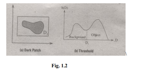
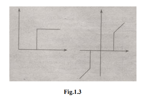
The figure 1.2 (b) consists of two peaks i.e., background and object. At the abscissa of histogram minimum (D1) the threshold is selected. This selected threshold (D1) can separate background and object to convert the image into its respective binary form. The thresholding transformations are shown in figure 1.3.
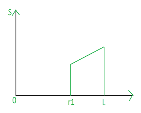
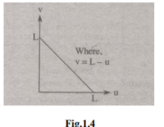
3. Digital Negative: The digital negative of an image is achieved by reverse scaling of its grey levels to the transformation. They are much essential in displaying of medical images. A digital negative transformation of an image is shown in figure 1.4.
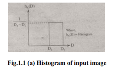
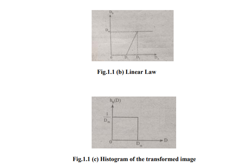
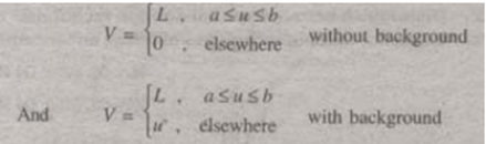
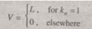
4. Intensity Level Slicing: The images which consist of grey levels in between intensity at background and other objects require to reduce the intensity of the object. This process of changing intensity level is done with the help of intensity level slicing. They are expressed as
The histogram of input image and its respective intensity level slicing is shown in the figure 1.5.
Then, the output is expressed as
Smoothing Frequency Domain filters
Ideal Lowpass Filter (ILPF)
ILPF is the simplest lowpass filter that “cuts off” all high frequency components of the DFT that are at a distance greater than a specifieddistance D0 from the origin of the (centered) transform.
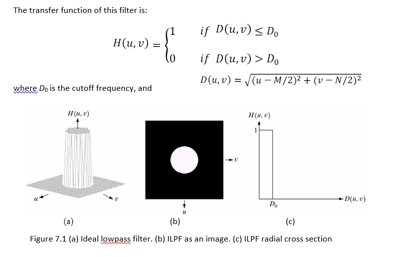
The ILPF indicates that all frequencies inside a circle of radius D0 are passed with no attenuation, whereas all frequencies outside this circle are completely attenuated.
The next figure shows a gray image with its Fourier spectrum. The circles super imposed on the spectrum represent cutoff frequencies 5, 15, 30, 80 and 230.
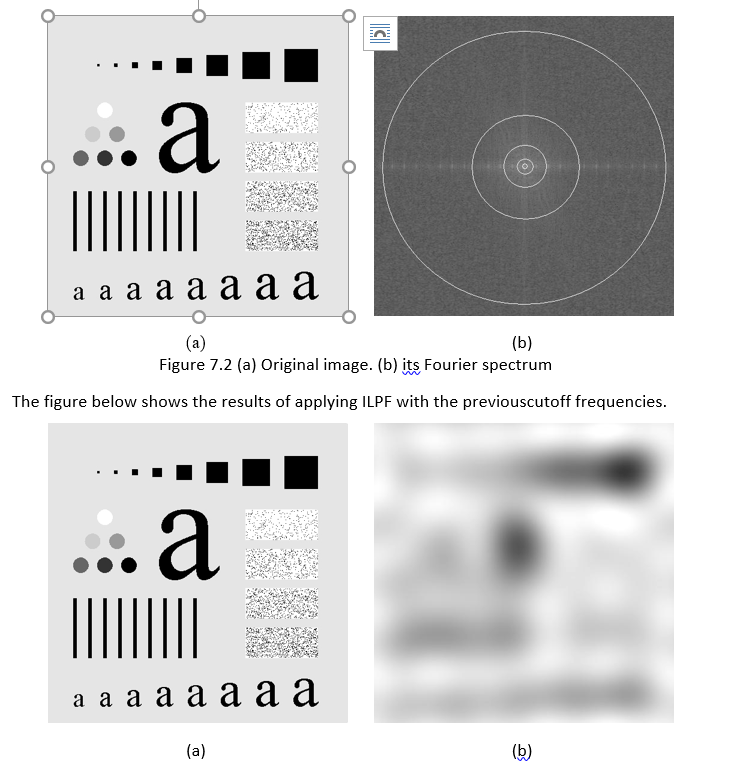
We can see the following effects of ILPF:
1. Blurring effect which decreases as the cutoff frequency increases.
2. Ringing effect which becomes finer (i.e. decreases) as the cutoff frequency increases.
Gaussian Lowpass Filter (GLPF)
The GLPF with cutoff frequency D0 is defined as:
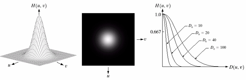
Unlike ILPF, the GLPF transfer function does not have a sharp transition that establishes a clear cutoff between passed and filtered frequencies.
Instead, GLPF has a smooth transition between low and high frequencies.
The figure below shows the results of applying GLPF on the image in Figure 7.2(a) with the same previous cutoff frequencies.
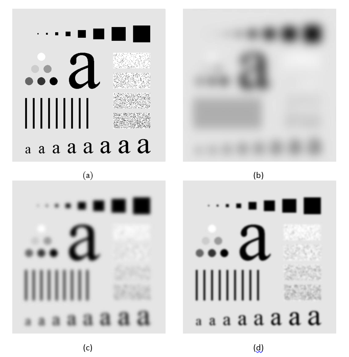
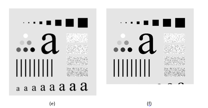
Figure 7.5 (a) Original image. (b) - (f) Results of GLPF with cutoff frequencies 5, 15, 30, 80, and 230 respectively.
We can see the following effects of GLPF compared to ILPF:
1. Smooth transition in blurring as a function of increasing cutoff frequency.
2. No ringing effect.
Smoothing (lowpass) filtering is useful in many applications. For example, GLPF can be used to bridge small gaps in broken characters by blurring it as shown below. This is useful for character recognition.
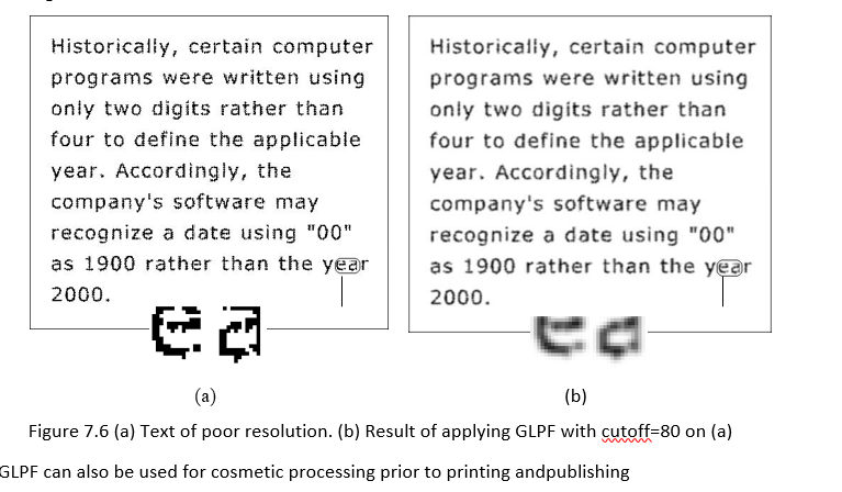
GLPF can also be used for cosmetic processing prior to printing and publishing
Sharpening Domain filters
Edges and sudden changes in gray levels are associated with high frequencies. Thus to enhance and sharpen significant details we need to use highpass filters in the frequency domain
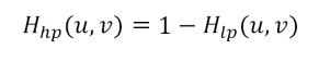
For any lowpass filter there is a highpass filter:
Ideal Highpass Filter (IHPF)
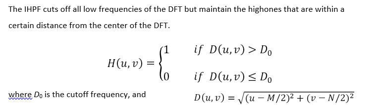
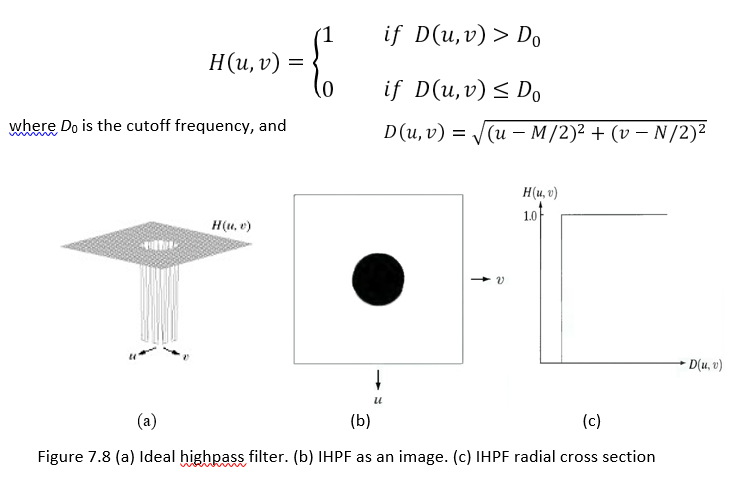
The IHPF sets to zero all frequencies inside a circle of radius D0 while passing, without attenuation, all frequencies outside the circle.
The figure below shows the results of applying IHPF with cutoff frequencies 15, 30, and 80.
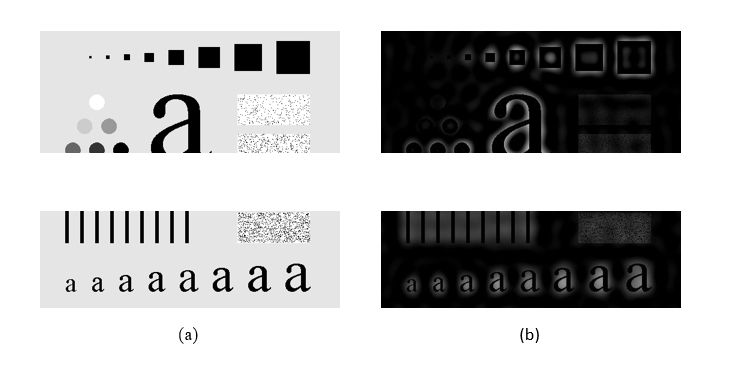
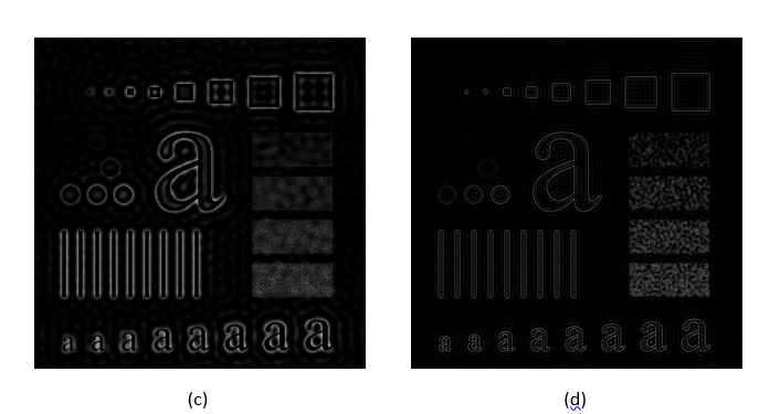
Figure 7.9 (a) Original image. (b) - (d) Results of IHPF with cutoff frequencies 15, 30, and 80 respectively.
We can see the following effects of IHPF:
1. Ringing effect.
2. Edge distortion (i.e. distorted, thickened object boundaries). Both effects are decreased as the cutoff frequency increases.
Gaussian Highpass Filter (GHPF)
The Gaussian Highpass Filter (GHPF) with cutoff frequency at distance
D0 is defined as:
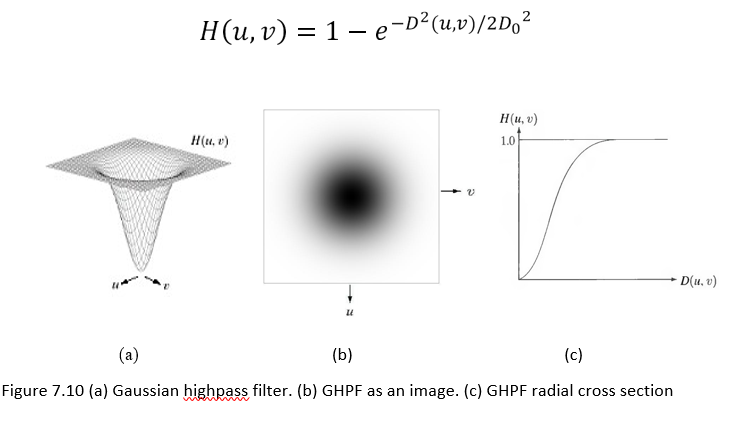
Figure 7.10 (a) Gaussian highpass filter. (b) GHPF as an image. (c) GHPF radial cross section
The figure below shows the results of applying GHPF with cutoff frequencies 15, 30 and 80.
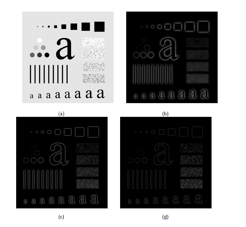
Figure 7.11 (a) Original image. (b) - (d) Results of GHPF with cutoff frequencies 15, 30, and 80 respectively.
The effects of GHPF in comparison with IHPF are:
1. No ringing effect.
2. Less edge distortion.
3. The results are smoother than those obtained by IHPF.
Homomorphic filtering.
Homomorphic filters are widely used in image processing for compensating the effect of no uniform illumination in an image. Pixel intensities in an image represent the light reflected from the corresponding points in the objects.
As per as image model, image f(z,y) may be characterized by two components: (1) the amount of source light incident on the scene being viewed, and (2) the amount of light reflected by the objects in the scene. These portions of light are called the illumination and reflectance components, and are denoted i ( x , y) and r ( x , y) respectively.
The functions i ( x , y) and r ( x , y) combine multiplicatively to give the image function f ( x , y): f ( x , y) = i ( x , y).r(x, y) (1) where 0 < i ( x , y ) < a and 0 < r( x , y ) < 1.
Homomorphic filters are used in such situations where the image is subjected to the multiplicative interference or noise as depicted in Eq. 1. We cannot easily use the above product to operate separately on the frequency components of illumination and reflection because the Fourier transform of f ( x , y) is not separable; that is F[f(x,y)) not equal to F[i(x, y)].F[r(x, y)].
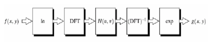
We can separate the two components by taking the logarithm of the two sides ln f(x,y) = ln i(x, y) + ln r(x, y). Taking Fourier transforms on both sides we get, F[ln f(x,y)} = F[ln i(x, y)} + F[ln r(x, y)]. that is, F(x,y) = I(x,y) + R(x,y), where F, I and R are the Fourier transforms ln f(x,y),ln i(x, y) , and ln r(x, y). respectively.
The function F represents the Fourier transform of the sum of two images: a low-frequency illumination image and a high-frequency reflectance image. If we now apply a filter with a transfer function that suppresses low- frequency components and enhances high-frequency components, then we can suppress the illumination component and enhance the reflectance component.
Features & Application:
1.Homomorphic filter is used for image enhancement.
2.It simultaneously normalizes the brightness across an image and increases contrast.
3.It is also used to remove multiplicative noise

