Model of image degrading/restoration process:

The principal goal of restoration techniques is to improve an image in some predefined sense. Restoration attempts to recover an image that has been degraded, by using a priori knowledge of the degradation phenomenon.

ii. Thus restoration techniques are oriented towards modelling the degradation and applying the inverse process in order to recover the original image.

iii. As Fig. 1 shows, the degradation process is modelled as a degradation function that, together with an additive noise term, operates on an input image f(x, y) to produce a degraded image g(x, y).

iv. Given g(x, y), some knowledge about the degradation function H, and some knowledge about the additive noise term f(x, y), the objective of restoration is to obtain an estimate f(x, y) of the original image.

v. We want the estimate to be as close as possible to the original input image and, in general, the more we know about H and f, the closer f(x, y) will be to f(x, y).

vi. The restoration approach used mostly is based on various types of image restoration filters

vii. We know that if H is a linear, position-invariant process, then the degraded image is given in the spatial domain by

g(x,y)=h(x,y)∗f(x,y)+77(x,y)      Eq.(1)

Where h(x, y) is the spatial representation of the degradation function and the symbol "*" indicates convolution.

viii. Now, convolution in the spatial domain is analogous to multiplication in the frequency domain, so we may write the model in Eq. (1) in an equivalent frequency domain representation:

G(u,v)=H(u,v)F(u,v)+N(u,v) (2)

ix. Where the terms in capital letters are the Fourier transforms of the corresponding terms in Eq. (1). These two equations are the bases for most of the restoration material.

x. This is about the basic image restoration model.

noise models (At the end of the pdf)

Restoration in the Present of Noise

When the only degradation present in an image is noise, i.e.

g(x,y)=f(x,y)+η(x,y) or G(u,v)= F(u,v)+ N(u,v)

The noise terms are unknown so subtracting them from g(x,y) or G(u,v) is not a realistic approach. In the case of periodic noise it is possible to estimate N(u,v) from the spectrumG(u,v).

So N(u,v) can be subtracted from G(u,v) to obtain an estimate of original image. Spatial filtering can be done when only additive noise is present. The following techniques can be used to reduce the noise effect:

i) Mean Filter:

ii) (a)Arithmetic Mean filter: It is the simplest mean filter. Let Sxy represents the set of coordinates in the sub image of size m*n centered at point (x,y). The arithmetic mean filter computes the average value of the corrupted image g(x,y) in the area defined by Sxy. The value of the restored image f at any point (x,y) is the arithmetic mean computed

using the pixels in the region defined by Sxy.

This operation can be using a convolution mask in which all coefficients have value 1/mn. A mean filter smoothes local variations in image Noise is reduced as a result of blurring. For every pixel in the image, the pixel value is replaced by the mean value of its neighboring pixels with a weight .This will resulted in a smoothing effect in the image.

(b)Geometric Mean filter:

An image restored using a geometric mean filter is given by the expression

This filter is useful for flinging the darkest point in image. Also, it reduces salt noise of the min operation.

(c)Midpoint filter: The midpoint filter simply computes the midpoint between the maximum and minimum values in the area encompassed by

It comeliness the order statistics and averaging .This filter works best for randomly distributed noise like Gaussian or uniform noise.

(d)Harmonic Mean filter: The harmonic mean filtering operation is given by the expression

The harmonic mean filter works well for salt noise but fails for pepper noise. It does well with Gaussian noise also.

(c) Order statistics filter: Order statistics filters are spatial filters whose response is based on ordering the pixel contained in the image area encompassed by the filter. The response of the filter at any point is determined by the ranking result.

Median filter:

It is the best order statistic filter; it replaces the value of a pixel by the median of gray levels in the Neighborhood of the pixel.

The original of the pixel is included in the computation of the median of the filter are quite possible because for certain types of random noise, the provide excellent noise reduction capabilities with considerably less blurring then smoothing filters of similar size. These are effective for bipolar and unipolor impulse noise.

Max and Min filter:

Using the l00th percentile of ranked set of numbers is called the max filter and is given by the equation

It is used for finding the brightest point in an image. Pepper noise in the image has very low values, it is reduced by max filter using the max selection process in the sublimated area sky. The 0th percentile filter is min filter

Linear Position-Invariant Degradations

Inverse filtering

The simplest approach to restoration is direct inverse filtering where we complete an estimate of the transform of the original image simply by dividing the transform of the degraded image G(u,v) by degradation functionH(u,v)

We know that

Therefore

From the above equation we observe that we cannot recover the undegraded image exactly because N(u,v) is a random function whose Fourier transform is not known.

One approach to get around the zero or small-value problem is to limit the filter frequencies to values near the origin.

We know that H(0,0) is equal to the average values of h(x,y). By Limiting the analysis to frequencies near the origin we reduce the probability of encountering zero values.

Minimum mean square error (Weiner) filtering.

The inverse filtering approach has poor performance. The wiener filtering approach uses the degradation function and statistical characteristics of noise into the restoration process.

The objective is to find an estimate of the uncorrupted image f such that the mean square error between them is minimized. The error measure is given by

Where E{.} is the expected value of the argument.

We assume that the noise and the image are uncorrelated one or the other has zero mean.

The gray levels in the estimate are a linear function of the levels in the degraded image.

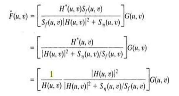
Where H(u,v)= Degradation function

H*(u,v)=complex conjugate of H(u,v)

| H(u,v)|²=H* (u,v) H(u,v)

Sn(u,v)=|N(u,v)|²= power spectrum of the noise

The power spectrum of the under graded image is rarely known. An approach used frequently when these quantities are not known or cannot be estimated then the expression used is

Where K is a specified constant

Color Image Processing

The use of color is important in image processing because:

· Color is a powerful descriptor that simplifies object identification and extraction.

· Humans can discern thousands of color shades and intensities, compared to about only two dozen shades of gray.

Color image processing is divided into two major areas:

· Full-color processing: images are acquired with a full-color sensor, such as a color TV camera or color scanner.

· Pseudocolor processing: The problem is one of assigning a color to a particular monochrome intensity or range of intensities.

Color Fundamentals

Colors are seen as variable combinations of the primary color s of light:red (R), green (G), and blue (B). The primary colors can be mixed to produce the secondary colors: magenta (red+blue), cyan (green+blue), and yellow (red+green). Mixing the three primaries, or a secondary with its opposite primary color, produces white light.

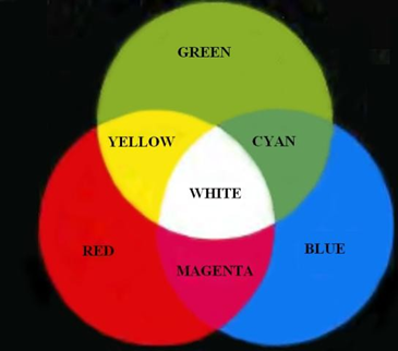
Figure 15.1 Primary and secondary colors of light

RGB colors are used for color TV, monitors, and video cameras.

However, the primary colors of pigments are cyan (C), magenta (M), and yellow (Y), and the secondary colors are red, green, and blue. A proper combination of the three pigment primaries, or a secondary with its opposite primary, produces black.

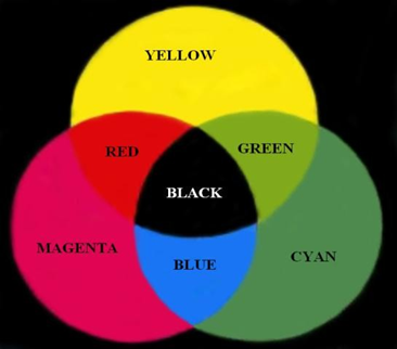
Figure 15.2 Primary and secondary colorsof pigments

CMY colors are used for color printing.

Color characteristics

The characteristics used to distinguish one color from another are:

·   Brightness: means the amountof intensity (i.e.color level).

·   Hue: represents dominant color as perceivedby an observer.

·   Saturation: refersto the amount of white light mixedwith a hue.

Color Models

The purpose of a color model is to facilitate the specification of colors in some standard way. A color model is a specification of a coordinate system and a subspace within that system where each color is represented by a single point. Color models most commonly used in image processing are:

·   RGB model for color monitorsand video cameras

· CMY and CMYK (cyan, magenta, yellow, black) models for color printing

·   HSI (hue, saturation, intensity) model

The RGB color model

In this model, each color appears in its primary colors red, green, and blue. This model is based on a Cartesian coordinate system. The color subspace is the cube shown in the figure below. The different colorsin this model are points on or inside the cube, and are defined by vectorsextending from the origin.

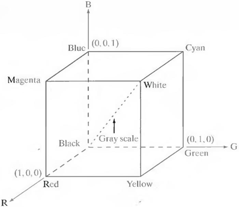
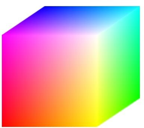
Figure 15.3 RGB color model

All color values R, G, and B have been normalized in the range [0, 1]. However, we can represent each of R, G, and B from 0 to 255.

Each RGB color image consists of three component images, one for each primary color as shown in the figure below. These three images are combined on the screen to produce a color image.

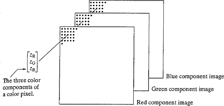
Figure 15.4 Scheme of RGB color image

The total number of bits used to represent each pixel in RGB image is called pixel depth. For example, in an RGB image if each of the red, green, and blue images is an 8-bit image, the pixel depth of the RGB image is 24-bits. The figure below shows the component images of an RGB image.

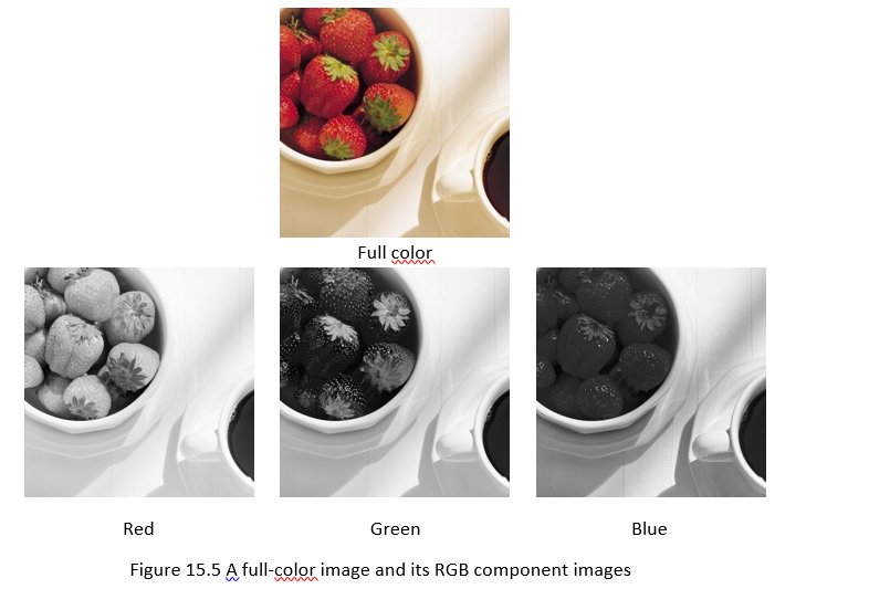
The CMY and CMYK color model

Cyan, magenta, and yellow are the primary colors of pigments. Most printing devices such as color printers and copiers require CMY data input or perform an RGB to CMY conversion internally. This conversion is performed using the equation

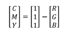
where, all color values have been normalized to the range [0, 1].

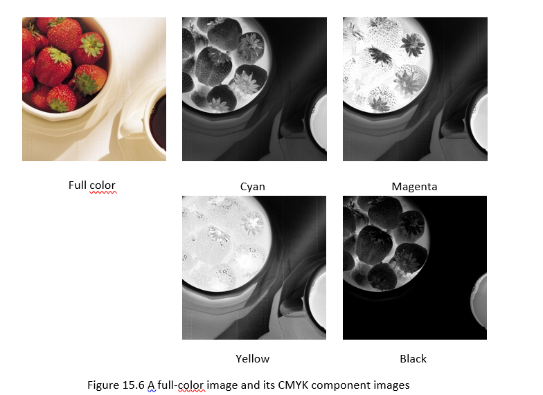
In printing, combining equal amounts of cyan, magenta, and yellow produce muddy-looking black. In order to produce true black, a fourth color, black, is added, giving rise to the CMYK color model.

The figure below shows the CMYK component images of an RGB image.

The HSI color model

The RGB and CMY color models are not suited for describing colors in terms of human interpretation. When we view a color object, we describe it by its hue, saturation, and brightness (intensity). Hence the HSI color model has been presented. The HSI model decouples the intensity component from the color-carrying information (hue and saturation) in a color image. As a result, this model is an ideal tool for developing color image processing algorithms.

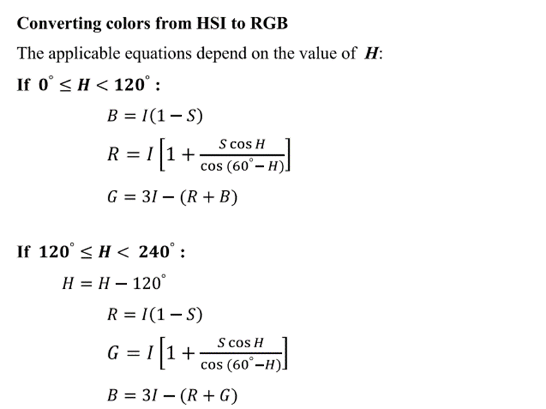
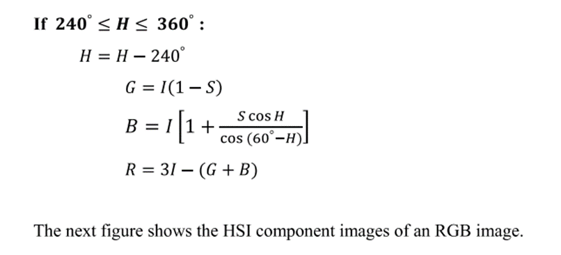
The hue, saturation, and intensity values can be obtained from the RGB color cube. That is, we can convert any RGB point to a corresponding point is the HSI color model by workingout the geometrical formulas.

Converting colors from RGB to HSI

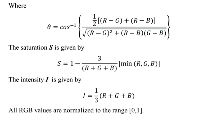
The hue H is given by

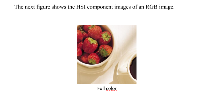
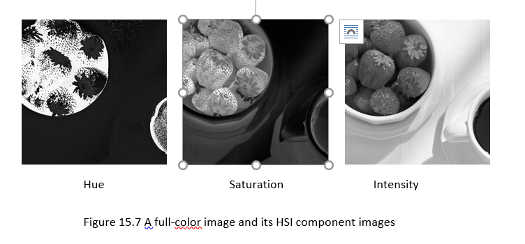
Basics of Full-Color Image Processing

Full-color imageprocessing approaches fall into two major categories:

· Approaches that process each component image individually and then form a composite processed color image from the individually processed components.

· Approachesthat work with color pixelsdirectly.

In full-color images, color pixels really are vectors. For example, in the RGB system,each color pixel can be expressed as

In order for per color component and vector based processing to be equivalent, two conditions have to be satisfied: First the process has to be applicable to both vectors and scalars. Second, the operation on each component of a vector must be independent of the other components.

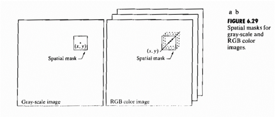
Fig 6.29 shows neighborhood spatial processing of gray-scale and full color images.

Suppose that the process is neighborhood averaging. In fig 6.29(a) averaging would be accomplished by summing the intensities of all the pixels in the neighbdorhood and dividing by the total number of pixels in the neighborhood.

Fig 6.29(b) averaging would be doneby summing all the vectors in the neighborhood and dividing each component by the total number of vectors in the neighborhood. But each component of the average vector is the sum of the pixels in the image corresponding to that component, which is the same as the result that would be obtained if the averaging were done on a per-color component basis and then the vector was formed

Color Transformation

As with the gray-level transformation, we model color transformations using the expression

(𝑥, 𝑦) = 𝑇[ƒ(𝑥, 𝑦)]

where f(x, y) is a color input image, g(x, y) is the transformed color output image, and T is the color transform.

This color transform can also be written

𝑠_i = 𝑇_i(𝑟₁, 𝑟₂, … , 𝑟_𝑛)                        i = 1,2, … , 𝑛

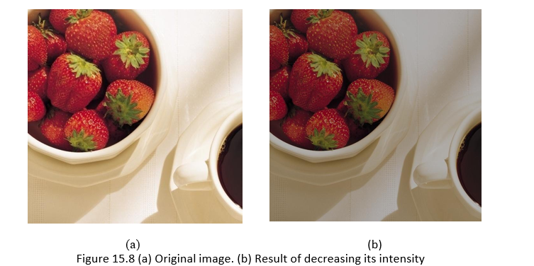
For example, we wish to modify the intensity of the image shown in Figure14.8(a) using

(𝑥, 𝑦) = 0.7ƒ(𝑥, 𝑦)

·   In the RGB color space, three components must betransformed:

𝑠_i = 0.7𝑟_i                 i = 1,2,3

·   In CMY space, also three component images must be transformed

𝑠_i = 0.7𝑟_i + 0.3                      i = 1,2,3

·   In HSI space, only intensity component𝑟₃istransformed

𝑠₃ = 0.7𝑟₃

Pseudocolor image processing

Pseudocolor (also called false color) image processing consists of assigning colors to gray values based on specific criterion. The term pseudo or false colour is used to differentiate the process of assigning colours in monochrome images from the processes associated with true colour images.The principal use of pseudocolor is for human visualization and interpretation of gray scale events in an image or sequence of images

Intensity Slicing

The technique of intensity (sometimes called density) slicing and colour coding is one of the simplest examples of pseudocolor image processing.

If an image is interepreted as a 3D function, the method can be viewed as one of placing planes parallel to the coordinate plane of the image; each plan then “slices: the function in the area of intersection. Figure 6.18 shows an example of using a plane at f(x,y) = l_i to slice the image function into two levels.

If a different color is assigned to each side of the plane shown in fig 6.18, any pixel whose intensity level is above the plane will be coded with one color, and any pixel below the plane will be coded with the other.

Levels that lie on the plane itself may be arbitrarily assigned one of the two colors. The result is a two color image whose relative appearance can be controlled by moving the slicing plane up and down the intensity axis.

In general the technique may be summarized as follows.

Let [0, L -1] represent the gray scale, Let [0, L – 1] represent the gray scale,

let level l₀ represent black [f(x,y) = 0] and level l_L-1 represent white [f(x,y) = L -1].

Suppose that P planes perpendicular to the intensity axis are defined at levels l₁, l₂… l_p. Then assuming that  0, P < L – 1, the P planes partition the gray scale into P + 1 intervals, V₁, V₂… V_{P + 1}.

Intensity to color assignments are made according to the relation

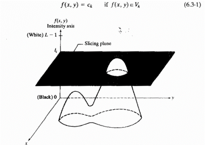
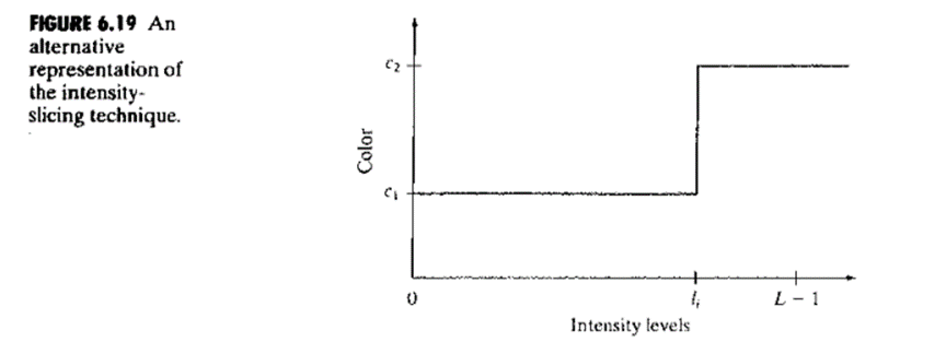
Fig 6.19 shows an alternative representation that defines the same mapping as in fig 6.18. According to the mapping functions shown in fig 6.19, any input intensity level is assigned one of two colours, depending on whether it is above or below the value of l_i.

When more levels are used, the mapping function takes on a staircase form

Intensity to Color Transformation

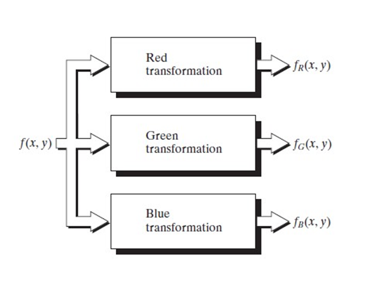
We can generalize the above technique by performing three independent transformations on the intensity of the image, resulting in three images which are the red, green, blue component images used to produce a color image. The three results are then fed separately into the red, green and blue channels of a color television monitor.

This method produces a composite image whose color content is modulated by the nature of the transformation functions.

The flexibility can be even more enhanced by using more than one monochrome images, for example, the three components of an RGB and the thermal image.

This technique is called multispectral image processing.

We often come across multispectral images in remote sensing systems, for example, Landsat Thematic Mapper (TM) Band 7 which targets the detection of hydrothermal
alteration zones in bare rock surfaces.

Multispectral image processing allows us to infer the wavelengths that cannot be captured by the conventional RGB cameras or even human eyes. This is an important technique for space-based images, or document and painting analysis.

Noise models

The principal source of noise in digital images arises during image acquisition and or transmission. The performance of imaging sensors is affected by a variety of factors, such as environmental conditions during image acquisition and by the quality of the sensing elements themselves. Images are corrupted during transmission principally due to interference in the channels used for transmission. Since main sources of noise presented in digital images are resulted from atmospheric disturbance and image sensor circuitry, following assumptions can be made i.e. the noise model is spatial invariant (independent of spatial location). The noise model is uncorrelated with the object function.

GAUSSIAN NOISE:

These noise models are used frequently in practices because of its tractability in both spatial and frequency domain.

The PDF of Gaussian random variable is

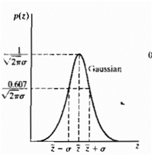
Where z represents the gray level, μ= mean of average value of z, σ= standard deviation.

Source of Gaussian Noise :

The Gaussian noise arises in an image due to factors such as electronic circuit noise and sensor noise due to poor illumination. The images acquired by image scanners exhibit this phenomenon.

RAYLEIGH NOISE:

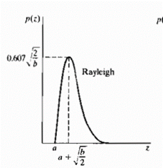
Unlike Gaussian distribution, the Rayleigh distribution is no symmetric. It is given by the formula

The mean and variance of this density is

(iii) GAMMA NOISE: The PDF of Erlang (Gamma)  noise is given by

The mean and variance of this density are given by

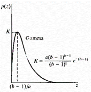
Its shape is similar to Rayleigh disruption. This equation is referred to as gamma density it is correct only when the denominator is the gamma function

(iv) EXPONENTIAL NOISE: Exponential distribution has an exponential shape.

The PDF of exponential noise is given as

Where a>0. The mean and variance of this density are given by

Exponential pdf is a special case of Erlang pdf with b =1.

Used in laser imaging.

(v)UNIFORM NOISE: The PDF of uniform noise is given by

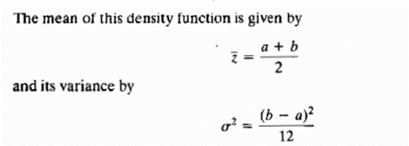
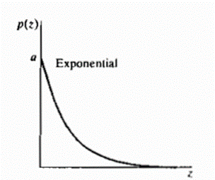
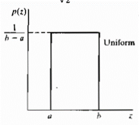
Figure 3.2.4 shows a plot of the Rayleigh density. Note the displacement from the origin and the fact that the basic shape of this density is skewed to the right. The Rayleigh density can be quite useful for approximating skewed histograms.

Impulse (salt-and-pepper) noise (bipolar) is specified as

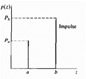
Figure shows a plot of the Rayleigh density. Note the displacement from the origin and the fact that the basic shape of this density is skewed to the right. The Rayleigh density can be quite useful for approximating skewed histograms

If b>a, intensity b will appear as a light dot on the image and a appears as a dark dot If either Pa or Pb is zero the noise is called unipolar. If neither probability is zero, and especially if they are approximately equal, impulse noise value will resemble salt and pepper granules randomly distributed over the image. For this reason, bipolar impulse noise is called salt and pepper noise.

In this case, the noise is signal dependent, and is multiplied to the image.