Electric Vehicles 1st Module

Module-1 Vehicle Mechanics:

Roadway Fundamentals

A vehicle moves on a level road and also up and down the slope of a roadway. We can simplify our description of the roadway by considering a straight roadway. Furthermore, we will define a tangential coordinate system that moves along with the vehicle, with respect to a fixed two-dimensional system.

The roadway description will be utilized to calculate the distance traversed by a vehicle along the roadway. The fixed coordinate system is attached to the earth such that the force of gravity is perpendicular to the unit vector vector t_Fvvand in the x_Fy_F plane. Let us consider a straight roadway, i.e., the steering wheel is locked straight along the X_F direction. The roadway is then in the x_Fy_F plane of the fixed coordinate system (Figure 2.1)

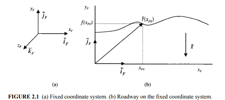
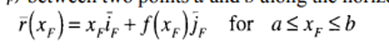
The two-dimensional roadway can be described as y_F=f(x_F). The roadway position vector

between two points a and b along the horizontal direction is

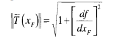
The distance-norm of the tangent vector

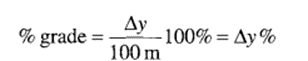
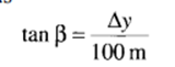
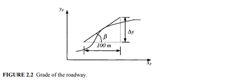
The roadway percent grade is the vertical rise per 100 horizontal distance of roadway, with both distances expressed in the same units. The angle β of the roadway associated with the slope or grade is the angle between the tangent vector and the horizontal axis X_F (Figure 2.2). If ∆y is the vertical rise in meters, then

The tangent of the slope angle is

The percent grade, or β, is greater than zero when the vehicle is on an upward slope and is less than zero when the vehicle is going downhill. The roadway percent grade can be described as a function of the roadway, as

Laws of Motion

Newton’s second law of motion can be expressed in equation form as follows:

Where

is the net force, m is the effective mass, and ā is the acceleration. The law is applied to the vehicle by considering a number of objects located at several points of contact of the vehicle with the outside world on which the individual forces act.

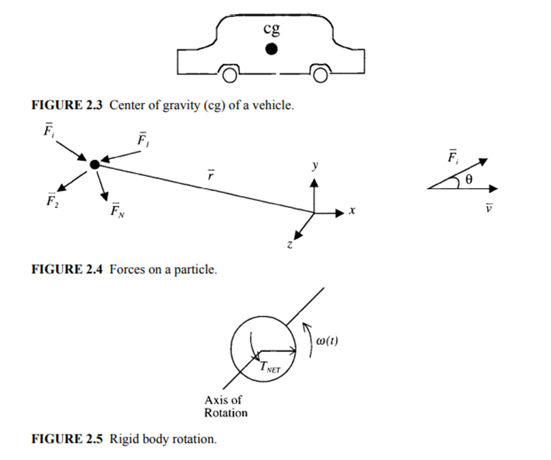
Examples of such points of contact are the front and rear wheels touching the roadway surface and vehicle, the frontal area that meets the force from air resistance, etc. We will simplify the problem by merging all of these points of contact into one location at the center of gravity (cg) of the EV and HEV, which is justified, because the extent of the object is immaterial. For all of the force calculations to follow, we will consider the vehicle to be a particle mass located at the cg of the vehicle. The cg can be considered to be within the vehicle, as shown in Figure 2.3.

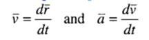
Particle motion is described by particle velocity and acceleration characteristics. For the position vector

for the particle mass on which several forces are working, as shown in Figure 2.4, the velocity v and acceleration a are

The power input to the particle for the ith force is

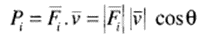
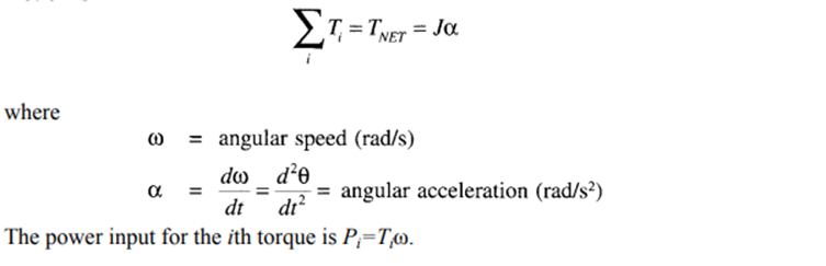
where θ is the angle between Fi and the resultant velocity v. For a rigid body rotating about a fixed axis, the equivalent terms relating motion and power are torque, angular velocity, and angular acceleration. Let there be i independent torques acting on a rigid body, causing it to rotate about an axis of rotation, as shown in Figure 2.5. If J (unit: kg-m²) is the polar moment of inertia of the rigid body, then the rotational form of Newton’s second law of motion is

Vehicle Kinetics

The tangential direction of forward motion of a vehicle changes with the slope of the roadway. To simplify the equations, a tangential coordinate system is defined below, so that the forces acting on the vehicle can be defined through a onedirectional equation. Let ū_T(x_F) be the unit tangent vector in the fixed coordinate system pointing in the direction of increasing X_F. Therefore

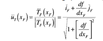
The tangential coordinate system shown in Figure 2.6 has the same origin as the fixed coordinate system. The z-direction unit vector is the same as that in the fixed coordinate system, but the x- and y-direction vectors constantly change with the slope of the roadway. Newton’s second law of motion can now be applied to the cg of EV in the tangential coordinate system as

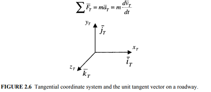
where m is the effective vehicle mass. The components of the coordinate system are:

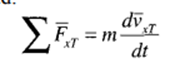
Component tangent to the road:

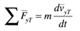
Component normal to the road:

And, because motion is assumed to be confined to the x_Ty_Tplane

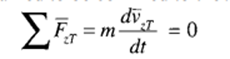
The vehicle tangential velocity is v_xT. The gravitational force in the normal direction is balanced by the road reaction force and, hence, there will be no motion in the y_T normal direction. In other words, the tire always remains in contact with the road.

The propulsion unit of the vehicle exerts a tractive force, F_TR, to propel the vehicle forward at a desired velocity. The tractive force must overcome the opposing forces, which are summed together and labeled as the road load force, F_RL. The road load force consists of the gravitational force, rolling resistance of the tires, and the aerodynamic drag force. The road load force is as follows:

where xT is the tangential direction along the roadway. The forces acting on the vehicle are shown in Figure 2.7.

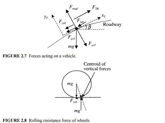
The rolling resistance is produced by the hysteresis of the tire at the contact surface with the roadway. In a stationary tire, the normal force to the road balances the distributed weight borne by the wheel at the point of contact along the vertical line beneath the axle. When the tire rolls, the centroid of the vertical forces on the wheel moves forward from beneath the axle toward the direction of motion of the vehicle, as shown in Figure 2.8. The weight on the wheel and the road normal force are misaligned due to the hysteresis of the tire. They form a couple that exerts a retarding torque on the wheel. The rolling resistance force, F_roll, is the force due to the couple, which opposes the motion of the wheel

Dynamics of Vehicle Motion

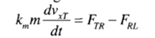
Tractive force is the force between the vehicle’s tires and the road (and parallel to the road) supplied by the electric motor in an EV and by the combination of electric motor and IC engine in an HEV to overcome the road load. The dynamic equation of motion in the tangential direction is given by

where k_m is the rotational inertia coefficient to compensate for the apparent increase in the vehicle’s mass due to the onboard rotating mass. The typical values of km are between 1.08 and 1.1, and it is dimensionless. The acceleration of the vehicle is dv_XT/dt.

Dynamic equations can be represented in the state space format for simulation of an EV or HEV system. The motion described by Equation 2.5 is the fundamental equation required for dynamic simulation of the vehicle system. One of the state variables of the vehicle dynamical system is v_xT.

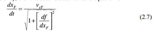
The second equation needed for modeling and simulation is the velocity equation, where either s or x_F can be used as the state variable. The slope of the roadway β will be an input to the simulation model, which may be given in terms of the tangential roadway distance as β=β(s) or in terms of the horizontal distance as β=β(x_F). If β is given in terms of s, then the second state variable equation is

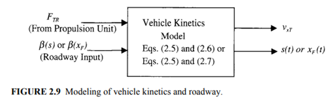
If β is given in terms of x_F, then the second state variable equation is

The input-output relational diagram for simulating vehicle kinetics is shown in Figure 2.9

Propulsion Power

The torque at the wheels of the vehicle can be obtained from the power relation:

where T_TR is the tractive torque in N-m, and ω_whis the angular velocity of the wheel in rad/s. F_TR is in N, and v_xTis in m/s. Assuming no slip between the tires and the road, the angular velocity and the vehicle speed are related by

where r_wh is the radius of the wheel in meters. The losses between the propulsion unit and wheels in the transmission and the differential have to be appropriately accounted for when specifying the power requirement of the propulsion unit.

An advantage of an electrically driven propulsion system is the elimination of multiple gears to match the vehicle speed and the engine speed. The wide speed range operation of electric motors enabled by power electronics control makes it possible to use a single gear-ratio transmission for instantaneous matching of the available motor torque T_motor with the desired tractive torque T_TR. The gear ratio and the size depend on the maximum motor speed, the maximum vehicle speed, the wheel radius, and the available traction between the tires and the road. A higher motor speed relative to the vehicle speed means a higher gear-ratio, larger size, and higher cost. However, higher motor speed is also desired in order to increase the power density of the motor. Therefore, a compromise is necessary between the maximum motor speed and the gear-ratio to optimize the cost. Planetary gears are typically used for EVs, with the gear-ratio rarely exceeding ten.

Force-Velocity Characteristics

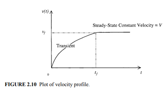
For an efficient design of the propulsion unit, the designer must know the force required to accelerate the vehicle to a cruising speed within a certain time and then to propel the vehicle forward at the rated steady state cruising speed and at the maximum speed on a specified slope. Useful design information is contained in the vehicle speed versus time and the steady state tractive force versus constant velocity characteristics, illustrated in Figures 2.10 and 2.11.

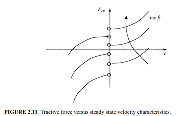
we will always assume the velocity to be in the tangential direction and denote it by v instead of v_xT for simplicity. The steady state constant velocity will be denoted by the uppercase letter V. Tractive force versus steady state velocity characteristics can be obtained from the equation of motion

When the steady state velocity is reached, dv/dt=0; and, hence, ΣF=0. Therefore, we have

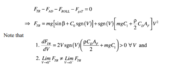
The first equation reveals that the slope of F_TRversus V is always positive, meaning that the force requirement increases as the vehicle speed increases, which is primarily due to the aerodynamic drag force opposing vehicle motion. Also, discontinuity of the curves at zero velocity is due to the rolling resistance force.

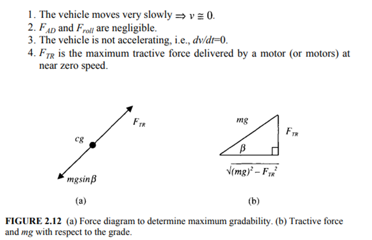
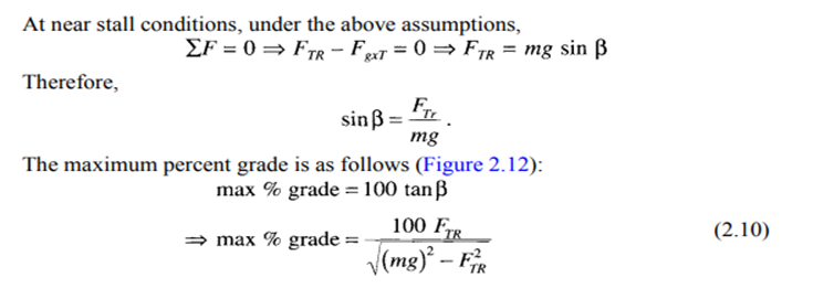
Maximum Gradability

The maximum grade that a vehicle will be able to overcome with the maximum force available from the propulsion unit is an important design criterion as well as performance measure. The vehicle is expected to move forward very slowly when climbing a steep slope and, hence, we can make the following assumptions for maximum gradability:

Velocity and Acceleration

The energy required from the propulsion unit depends on the desired acceleration and the road load force that the vehicle has to overcome.

Maximum acceleration is limited by the maximum tractive power available and the roadway condition at the time of vehicle operation. Although the road load force is unknown in a realworld roadway, significant insight about the vehicle velocity profile and energy requirement can be obtained through studies of assumed scenarios.

Vehicles are typically designed with a certain objective, such as maximum acceleration on a given roadway slope in a typical weather condition. Discussed in the following are two simplified scenarios that will set the stage for designing EVs and HEVs.

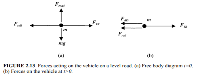
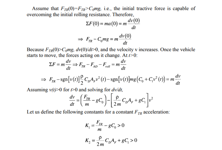
Constant FTR,Level Road

In the first case, we will assume a level road condition, where the propulsion unit for an EV exerts a constant tractive force. The level road condition implies that β (s) =0. We will assume that the EV is initially at rest, which implies v(0)=0. The free body diagram at t=0 is shown in Figure 2.13.

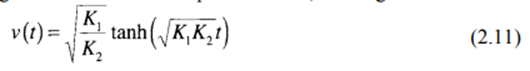
Velocity Profile

The velocity profile for the constant F_TR level road case (Figure 2.14) can be obtained by solving for v from the dv/dt equation above, which gives

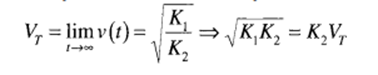
The terminal velocity can be obtained by taking the limit of the velocity profile as time approaches infinity. The terminal velocity is

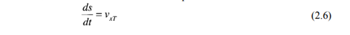
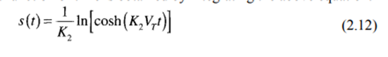
Distance Traversed

The distance traversed by the vehicle can be obtained from the following relation:

The distance as a function of time is obtained by integrating the above equation:

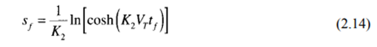
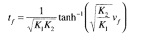
The starting acceleration is often specified as 0 to v_fm/s in t_fs, where v_f is the desired velocity at the end of the specified time t_fs. The time to reach the desired velocity is given by

and the distance traversed during the time to reach the desired velocity is given by

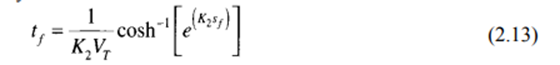
The desired time can also be expressed as follows:

where v_f the velocity after time t_f

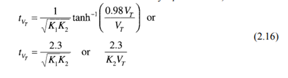
Let t_VT=time to reach 98% of the terminal velocity V_T. Therefore

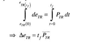
Tractive Power

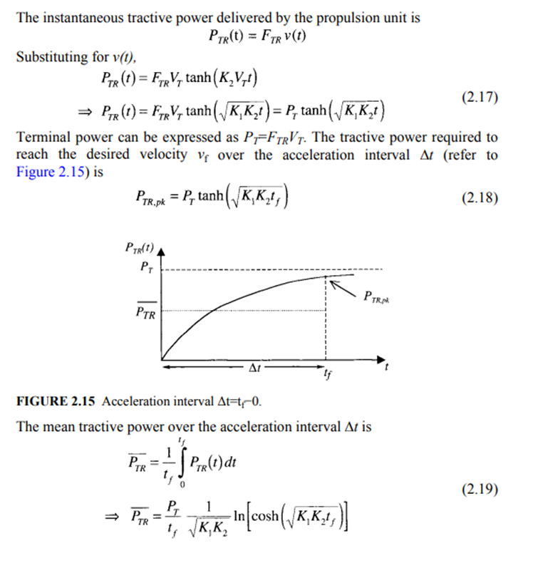
Energy Required

The energy requirement for a given acceleration and constant steady state velocity is necessary for the design and selection of the energy source or batteries to cover a certain distance. The rate of change of energy is the tractive power, given as

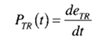
where e_TR is the instantaneous tractive energy. The energy required or energy change during an interval of the vehicle can be obtained from the integration of the instantaneous power equation as

Nonconstant FTR,General Acceleration

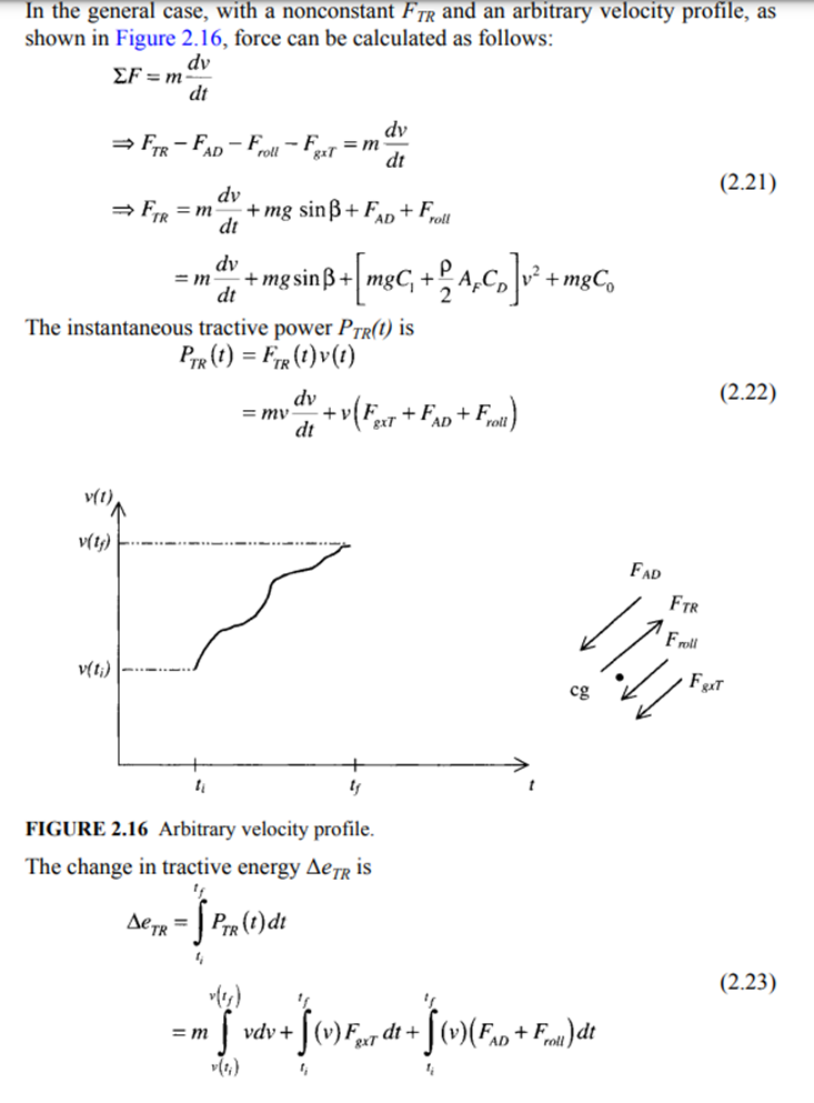
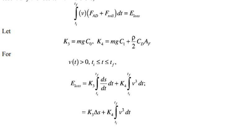
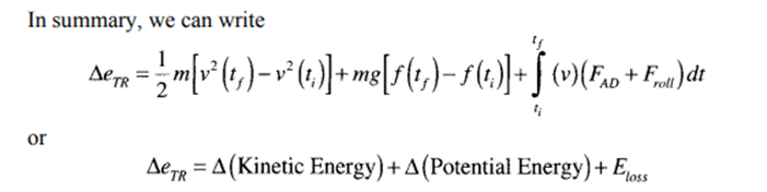
The energy supplied by the propulsion unit is converted into various forms of energy, some of which are stored in the vehicle system, while others are lost due to non-constructive forces. It is interesting to note the type of energy associated with each term in Equation 2.23. Let us consider the first term on the right side of Equation 2.23:

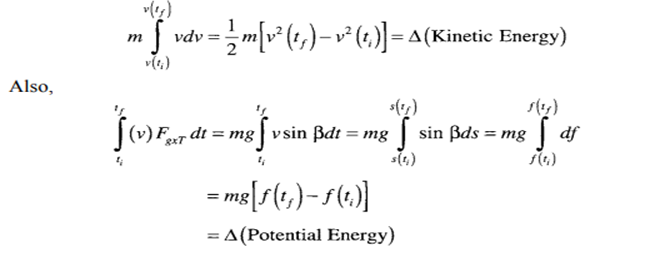
The above term represents change in vertical displacement multiplied by mg, which is the change in potential energy. The third and fourth terms on the right side of Equation 2.23 represent the energy required to overcome nonconstructive forces that include rolling resistance and aerodynamic drag force. The energy represented in these terms is essentially the loss term. Therefore,

Propulsion System Design.

The steady state maximum velocity, maximum gradability, and velocity equations can be used in the design stage to specify the power requirement of a particular vehicle. The common design requirements related to vehicle power expected to be specified by a customer are the initial acceleration, rated velocity on a given slope, maximum % grade, and maximum steady state velocity

The complete design is a complex issue involving numerous variables, constraints, considerations, and judgment.

Let us consider the tractive power requirement for initial acceleration, which plays a significant role in determining the rated power of the propulsion unit. The initial acceleration is specified as 0 to v_fin t_f s. The design problem is to solve for F_TR, starting with a set of variables including vehicle mass, rolling resistance, aerodynamic drag coefficient, percent grade, wheel radius, etc., some of which are known, while others have to be assumed. The acceleration of the vehicle in terms of these variables is given by

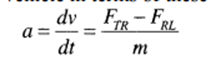
The tractive force output of the electric motor for an EV or the combination of electric motor and IC engine for an HEV will be a function of vehicle velocity. Furthermore, the road load characteristics are a function of velocity, resulting in a transcendental equation to be solved to determine the desired tractive power from the propulsion unit. Other design requirements also play a significant role in determining tractive power.