Micro and Smart System Technology 5th Module

Module 5- Implementation of Controllers for MEMS & Case Studies of Integrated Microsystems.

Design Methodology

The design of a control system involves locating the poles at appropriate positions so that the system response satisfies specified requirements and at the same time ensures the stability of the system.

The design of control system thus involves the design of a suitable compensation to modify the response of a plant in order that the stability of the system is ensured. Stability analysis is a very important preliminary step that determines how stable or unstable the system is and indicates to the designer the kind and amount of compensation necessary to ensure stability.

The second step in the design process is to analytically determine the parameters for the compensator. As mentioned earlier, an unstable system will have roots in the right half of the s-plane, and to stabilize the same we need to move these roots to the left half of the s-plane. In general, one can move the roots by

1. Changing gain.

2. Changing plant.

3. Placing a dynamic element in the forward transmission path.

4. Placing a dynamic element in the feedback path.

5. Feed back all or some of the states.

However, in practice the first two cases are seldom permissible. Hence, the design of a good control system involves addition of an element with a gain in the control loop. The gain of a control system can be a constant or a variable depending upon the control system design. The basic or minimum system is determined by having a closed loop with unity feedback.

Normally, sensors are assumed ideal and only an amplifier is added between the error signal and the plant. The gain is then set accordingly to meet the steady-state response and bandwidth requirements, and is dictated by the stability analysis.

PID controller

PID controller is a Close loop system which has feedback control system and it compares the Process variable (feedback variable) with set Point and generates an error signal and according to that it adjusts the output of system. This process continues until this error gets to Zero or process variable value becomes equal to set point.

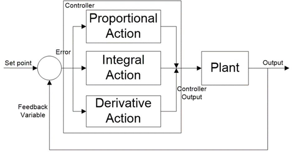
PID controller is a combination of three terms; Proportional, Integral and Derivative. Let us understand these three terms individually.

PID Modes of Control:

Proportional (P) response:

Term ‘P’ is proportional to the actual value of the error. If the error is large, control output is also large and if the error is small control output is also small, but gain factor (K_p) is

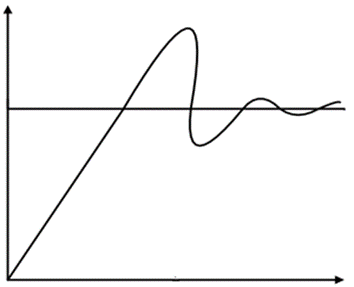
Also taking in to account. Speed of response is also directly proportional to proportional gain factor (K_p). So, the speed of response is increased by increasing the value of K_p but if K_p is increased beyond normal range, process variable starts oscillating at high rate and make system unstable.

PID controller Proportional response

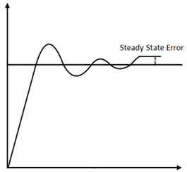
Here, the resulting error is multiplied with proportionality gain factor (proportional constant) as shown in above equation. If only P controller is used, at that time, it requires manual reset because it maintain steady state error (offset).

Integral (I) response:

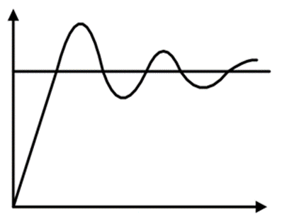
Integral controller is generally used to decrease the steady state error. Term ‘I’ is integrate (with respect to time) to the actual value of the error. Because of integration, very small value of error, results very high integral response. Integral controller action continues to change until error becomes zero.

PID controller Integral response

Integral gain is inversely proportional to the speed of response, increasing k_i, decrease the speed of response. Proportional and Integral controllers are used combined (PI controller) for good speed of response and steady state response.

Derivative (D) response:

Derivative controller is used to with combination of PD or PID. It never used alone, because if error is constant (non-zero), output of the controller will be zero. In this situation, controller behave life zero error, but in actual there are some error (constant). Output of derivative controller is directly proportional to the rate of change of error with respect to time

PID controller Derivative response

Proportional and Integral controller:

This is a combination of P and I controller. Output of the controller is summation of both (proportional and integral) responses. Mathematical equation is as shown in below;

Proportional and Derivative controller: This is a combination of P and D controller. Output of controller is summation of proportional and derivative responses.

Proportional, Integral and Derivative controller: This is a combination of P, I and D controller. Output of controller is summation of proportional, integral and derivative responses. Mathematical equation of PD controller is as shown below;

Thus, by combining this proportional, integral and derivative control response, form a PID controller.

Advantages:

1. It only acts on the error between the desired signal and the controlled signal. Hence, no extra measurements of the internal states are needed, which is one of the biggest advantage in applications because ….. more measurements mean more sensors, more signal conditioning, more maintenance, more cost.

2. Apart from certain structural properties of the plant/process, not much knowledge of the plant is required for tuning. The tuning can be done through trial and error or a look-up table. Not much expertise is needed for tuning, hence, few middle-skilled technicians may easily carry out the task….again cost cutting

3. It is efficient and robust against some common uncertainties if properly tuned (around an operating region).

4. Easy to implement in hardware (through filters) and also easy to implement though microcontrollers, PLC etc. No fancy codes to design… can be written by a middle-level programmer.

Disadvantages: cost is high, Complexity and tuning, design complexity.

Applications: Temperature Control of Furnace, MPPT Charge Controller, The Converter of Power Electronics, Closed Loop Control for a Brushless DC motor ,PID Controller Interfacing

Circuit Implementation

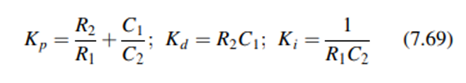
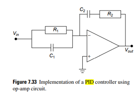
Controllers designed by the procedure discussed in the above paragraphs may be implemented in several ways. A simple op-amp circuit for implementing PID controller is shown in Figure 7.33. The transfer function for this circuit is given by

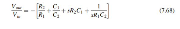
The corresponding control coefficients for this circuit are

Digital Controllers

Control systems using various forms of digital devices as the controller may be classified as digital control systems. The controller used in these may range from a microcontroller to an ASIC to a personal computer.

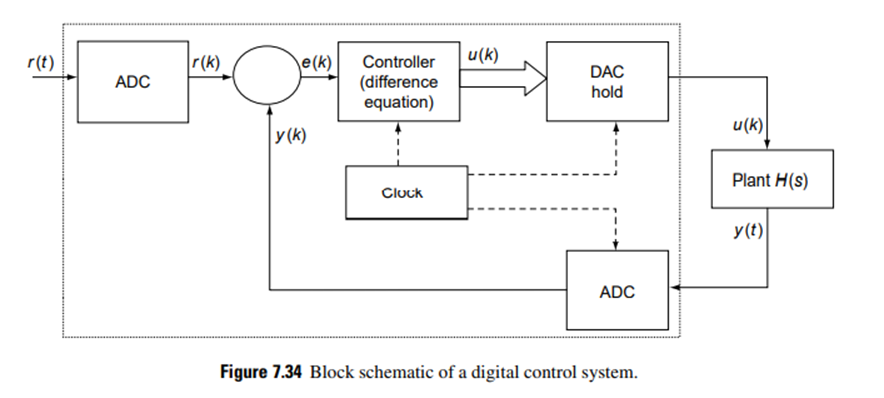
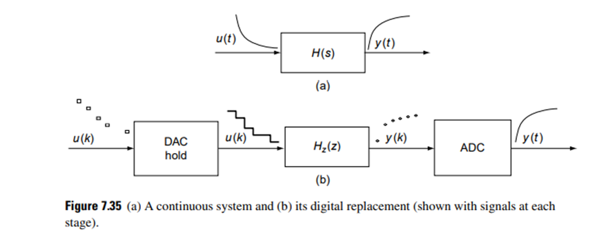
These digital systems operate on discrete signals that are samples of the sensed signal, rather than on continuous signals. Since most parameters in a plant operating continuously would vary continuously, DACs and ADCs are required in the implementation of such digital controllers. However, several additional blocks, as shown in Figure 7.34, are required to replace a continuous controller by a digital controller.

In Figure 7.34, the clock connected to the DACs and ADCs sends out pulses at a periodic interval T, which in turn makes these converters send their output signals to ensure that the controller output is synchronized with the feedback from the plant.

In this digital system design, a discrete function H_z(z) must be found so that, for a piecewise constant input to the continuous system H(s), the sampled output of the continuous system equals the discrete output. This is illustrated in Figure 7.35.

Microcontroller

A microcontroller-based design would be appropriate in large-volume production scenarios and where the end user does not need to alter the control. As is evident from the block schematic in Figure 7.36, a microcontroller is a small computer on a single chip consisting of CPU, clock, timers, I/O ports, and memory.

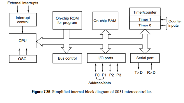
In general, microcontrollers are simple computers with low power consumption, usually operating at low clock speeds, typically designed for dedicated but low-computation-intensity applications.

Such a level of integration helps in drastically reducing the number of chips and printed circuit board space. Applications include control of implantable medical devices and airbag deployment systems in automobiles

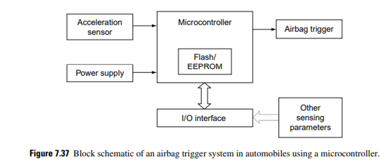
The application of microcontrollers in the triggering mechanism of airbags in automobiles is illustrated by the simplified schematic in Figure 7.37. When a crash happens, the inputs from the acceleration (deceleration) sensor are compared with a predefined set of parameters (based on other sensor data available from the onboard network), and the microcontroller evaluates the situation and takes the decision to activate the airbag triggers

PLC

Another variant of the digital controller is a programmable logic controller (PLC) used in automation of a plant or a smart system operating at severe environmental and/or process conditions. Like the microcontroller, the PLC is also designed for multiple input and output arrangements, but with extended operating temperature ranges and immunity to electrical noise.

Unlike microcontrollers that operate at 5 V or less, PLCs typically have a supply voltage requirement of 24 V. Control through them is typically simple and linear and does not usually depend on history of variation in the control variable. PLCs usually have logic for single-variable feedback control loop with a proportional, integral derivative or PID controller

PLCs are specifically suited for severe operating conditions such as dust, moisture, temperature, heat, or vibration. Its I/O interface may be either built in or via external I/O modules of a network including the PLC.

Case Studies of Integrated Microsystems: BEL pressure sensor

One of the first sensors fabricated using micromachining techniques was the pressure sensor. These are widely used in aerospace, automobile, biomedical, and defense applications. In general, pressure sensors are based on measuring the mechanical deformation caused in a membrane when it experiences stress due to pressure of a fluid. It may be noted that silicon is brittle and breaks at a maximum strain of 2%. However, its Young’s modulus is very high (190 GPa), and below the elastic limit strain is linearly related to stress.

The resulting strain or displacement (which is a measure of the pressure on the membrane) is converted to electrical signals. Several principles are used to sense strain: piezoelectricity, piezoresistivity, changes in capacitance, changes in resonant frequency of vibrating elements in the structure, and changes in optical resonance.

Most conventional pressure sensors use strain gauges. These sensors use the change in the resistance of conductors due to the change in their physical dimensions (deformations) when subjected to strain. These are attached to the membrane and give information about the strain experienced by the membrane due to the applied pressure.

However, if these sensors are made of semiconductors, the change in the resistance is predominantly due to a change in resistivity rather than to deformations. This effect, known as piezoresistivity, is a phenomenon by which the electrical resistance of a material changes in response to mechanical stress. In piezoresistive pressure sensors, semiconductor resistors are laid out on a membrane to sense the strain from the membrane that is subjected to external pressure.

The first piezoresistive pressure sensor based on diffused resistors in a thin silicon diaphragm was demonstrated in 1969. Piezoresistive pressure sensors are simple to fabricate and provide a directly readable electrical output. Further, they can be easily integrated with microelectronics circuits, since the fabrication processes are compatible with IC fabrication techniques. Therefore, we focus our discussion on piezoresistive pressure sensors.

Design Considerations of a Piezoresistive Pressure Sensor

The piezoresistive effect can be quantified using the gauge factor. The resistance of a rectangular conductor is expressed by

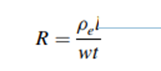
where Pe is the resistivity and l, w, and t are the length, width, and thickness of the conductor, respectively.

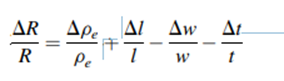
When the resistor is subjected to strain, the relative change in resistance is given by

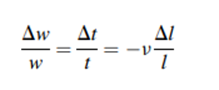
If the resistors experience tensile stress along the length, the resistor’s thickness and width decrease whereas the length increases. Poisson’s ratio, n, relates the change in length to the change in width and thickness of the piezoresistors by the following equation

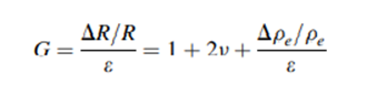
The gauge factor G (strain sensitivity) is given by

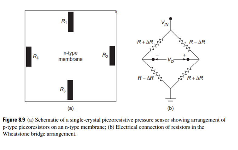
The basic structure of a piezoresistive pressure sensor consists of four sensing elements connected in a Wheatstone bridge configuration to measure stress in a thin membrane (see Figure 8.9). When fabricated using silicon bulk micromachining by anisotropic etching, the membrane is invariably rectangular or square and is realized on (100) plane with the edges in the directions. The stress is a direct consequence of the membrane deflection in response to an applied pressure. Therefore, the design of a pressure sensor involves (a) determination of the thickness and geometrical dimensions of the membrane and (b) location of the piezoresistors on the membrane to achieve maximum sensitivity.

Performance Parameters of Pressure Sensors

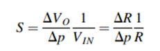
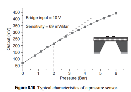
A typical response (output voltage of the Wheatstone bridge versus the pressure) of a pressure sensor in the literature is shown in Figure. The sensitivity S is defined as the relative change of output voltage per unit change of applied pressure (slope of the linear portion of the curve in Figure). This is expressed in mV/bar (1 bar=10⁵ Pascal) for a given input voltage. To be specific, sensitivity can also be expressed in mV/V/bar as:

The offset voltage (VOFF) is the output voltage of the pressure sensor when the applied pressure is zero. An offset voltage of about 65mV can be seen in the performance curve in Figure. This is mainly due to some residual stress on the membrane or variability in the four resistors. It can be compensated by using external resistors along with signal conditioning electronics.

The offset voltage (VOFF) is the output voltage of the pressure sensor when the applied pressure is zero. An offset voltage of about 65mV can be seen in the performance curve in Figure. This is mainly due to some residual stress on the membrane or variability in the four resistors. It can be compensated by using external resistors along with signal conditioning electronics.

The output voltage does not vary linearly with pressure when the applied pressure exceeds a certain value.

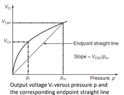
Nonlinearity is defined with reference to the full-scale output corresponding to the maximum pressure at which the sensor can be used. This can be better appreciated by referring to the output voltage VO versus applied pressure p and the endpoint straight line in Figure; the nonlinearity NL_i of a pressure sensor at a specific pressure pi is defined as follows:

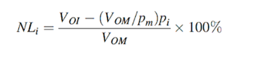
where VO_I and VO_M are respectively the output voltages at a pressure pi and the full-scale output voltage at the maximum pressure input p_m. Thus, the nonlinearity can be either positive or negative depending upon the calibration point. The nonlinearity of the pressure sensor is the maximum value of NL_i.

Nonlinearity in the piezoresistive pressure sensors is caused mainly by the following:

1. The nonlinear relationship between stress and applied pressure.

2. The piezoresistive coefficient of silicon is generally considered to be independent of stress. In practice, however, this

is not really true at high accuracy.

3. A difference in piezoresistive sensitivity between the resistors of the Wheatstone bridge.

CASE STUDY OF A SMART STRUCTURE IN VIBRATION CONTROL

➢The control of noise generated by vibration of structural members is yet another application where smart materials can be used. This has great impact in increasing the integrity of the structure.

➢Noise can be airborne or structure-borne. Airborne noises are generated due to the pressure difference caused by differential flow fields, as for example the aerodynamic noise generated by a moving aircraft or helicopter.

➢The structure borne noise is generated by vibrating structural members. These members act as a conduit for the vibration (disturbance) to propagate within the structure and are responsible for screeching or high-frequency noise.

➢In such cases, reducing the vibration levels automatically reduces the structure-borne noise levels.

PZT Transducers

➢ Piezoelectricity is attributed to an asymmetry in the unit cell and the resultant generation of electric polarization dipoles due to the mechanical distortion.

➢ Examples of piezoelectric materials include lead zirconate titanate (more popularly known by the acronym PZT), lead metaniobate, lead titanate, and their modifications. The changes in electrical charge are generated when mechanical stresses are applied across the face of a piezoelectric sheet or film. The converse effect is also observed in such materials.

➢ PZT is arguably the most widely used component in smart systems. Its importance comes from its substantial piezoelectric properties.

➢ In these crystals, the force applied along one axis of the crystal leads to the appearance of positive and negative charges on opposite sides of the crystal along another axis. The strain induced by the force F leads to a physical displacement of the charge Q within the unit cell. This polarization of the crystal leads to an accumulation of charge: Q = d F

➢ In general, forces in the x-, y- and z-directions contribute to charges produced in any of the three directions. Hence, the piezoelectric coefficient d is a 3x3 matrix. Values of the piezoelectric coefficients of these materials are usually made available by the manufacturer.

➢ Typical values of the piezoelectric charge coefficients are 1–100 pC/N. The reverse effect is used  in piezoelectric actuators. Application of voltage across such materials results in dimensional changes of the crystal. The change in length dL per unit applied voltage is given by

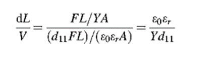
Here A is the cross-sectional area, L is the length of the beam, and d11 is the piezoelectric coefficient. Strain in this expression depends only on the piezoelectric coefficient, the dielectric constant, and Young’s modulus. Therefore, it may be inferred that objects of a given piezoelectric material, irrespective of its shape, undergo the same fractional change in length upon application of a given voltage.

➢ The relationship between dipole moment and mechanical deformation is expressed as constitutive relations:

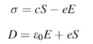
where σ is the mechanical stress, S the strain, E the electric field, D the flux density, c the elastic constant, e the piezoelectric constant, and ɛ0 the permittivity of free space. It may be noted that in the absence of piezoelectricity these relations reduce to Hooke’s law and the constitutive relation for dielectric materials, respectively.

Vibrations in Beams

➢ In this case study, vibration levels in a beam modeled by a thin-walled box are controlled using PZT actuators. Further the possibility of selecting the coefficients for a controller for any process or system can be done by following a few tuning steps. It was also shown that simple op-amp-based circuits can be designed to have the desired transfer function. Proportional-integral derivative (PID) controllers can also be digitally implemented with microprocessors.

An experimental structure of a glass-epoxy composite box beam with two bimorph surface-mounted PZT patches is shown in Figure. Such thin-walled geometries are used extensively in aircraft structural components due to their inherent advantage of high stiffness and low weight.

➢ They are also used in many steel structures such as girders, bridges, scaffolds, etc. Analysis of these structures involves secondary effects such as warping, ovaling, etc. In addition, thin-walled structures in aircraft can produce coupled motions, such as bending, giving rise to torsional motion.

Here we want to suppress transverse bending modes. The PZT patches act as actuators through which both the exciting electrical load and the control signals are applied.

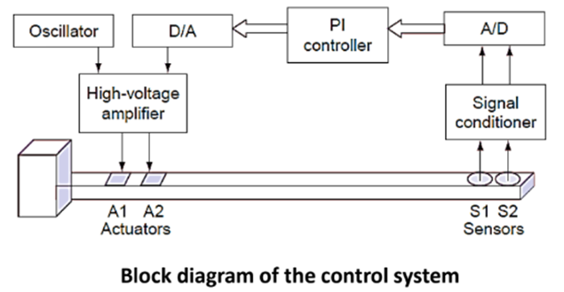
➢ The vibration in the box beam is induced through a single patch of PZT actuator using an oscillator. The generated vibration is sensed through an accelerometer that is then fed to the A/D converter after signal conditioning.

➢ The PI controller in this case can be implemented in a digital signal processing (DSP)-based control card. The sensed voltage is proportional to the acceleration; the control voltage from the controller is amplified by a high-voltage amplifier and then fed into the PZT actuators for bending actuation to suppress the transverse vibration.

➢First the closed-loop responses using PI controller are obtained using a SISO system and a single-output two-input system. The test specimen is excited in transverse bending mode by applying a single- frequency sinusoidal voltage through PZT actuators.

➢ Vibration suppression is performed by the PI controller. In this case, the tip acceleration is measured and the feedback is given as proportional gain KP times tip acceleration measured by theaccelerometer sensor S1.

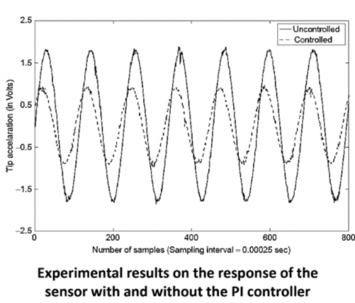
➢ In addition, an integral gain KI times the velocity of the tip (obtained by integrating its acceleration) is also included in the feedback. A sinusoidal voltage is applied through actuator A1 and the control signal is fed back through actuator A2. Kp and Ki values used can be obtained by tuning using the Ziegler–Nichols rule. The experimental results in Figure indicate significant suppression of vibrations in the beam.